
ハルビン工業大学(深圳)• 2024 • 入門計量経済学 Homework & Lab • における解決策 • HITSZ 基础计量经济学作业 • 实验 2024
当サイト内のコンテンツの無断転載、引用、コピーは禁止されています。
For those titles or questions with at least one ‘+’ mark, it shows that the corresponding part is of the course numbered “ECON2010” as an extra part than “ECON2010F”, which is an easier alternative Introductory Econometrics course.
Homework 1
1 : [15 points : Theory]
Remind yourself of the terminology we developed in Chapter 1 for causal questions. Suppose we are interested in the causal effect of having health insurance on an individual’s health status.
(a) [2 points] We run a phone survey where we ask 5,000 respondents about their current insurance and health conditions. The data we collect is an example of a __________.
(b) [2 points] The US government has Census data on every elderly American’s current insurance and health status. This is an example of data for the __________.
(c) [2 points] Suppose we take our phone survey data and calculate the difference in health between individuals who do and do not have insurance. This difference is an example of an __________.
(d) [4 points] The difference in health between all Americans who do and don’t have insurance is an example of an __________. The effect of insurance on health is an example of a __________.
(e) [5 points] When the two objects in (d) coincide, we have an example of __________. Give one reason why the two objects in (d) might not coincide.
Solution to (a)
sample
Solution to (b)
population
Solution to (c)
estimate (or estimator)
Solution to (d)
estimand
(target) parameter
Solution to (e)
identification
We might expect richer individuals to be more likely to have health insurance and more likely to be healthy for other reasons. In this case the difference in health of Americans with/without health insurance is likely to overstate the causal effect of insurance (upward selection bias).
2 : [25 points : Theory]
Let $Y=a+X^{3}/b$ where $a$ and $b$ are some constants with $b>0$, and where $X\sim\mathrm{N}(0,1)$.
(a) [2 points] State the definition of the cumulative density function of $Y$, which we’ll call $F_{a,b}(y)$.
(b) [5 points] Express $F_{a,b}(y)$ in terms of the CDF of the standard normal distribution $\Phi(\cdot)$. Hint: can you re-write the inequality $Y\le y$ as an inequality involving $X$?
(c) [3 points] Express $E[Y]$ in terms of $E[X^{3}]$, then use the fact that $E[X^{3}]=0$ when $X\sim\mathrm{N}(0,1)$ to derive $E[Y]$.
(d) [4 points] Express $Cov(Y,X)$ in terms of $E[X^{4}]$, then use the fact that $E[X^{4}]=3$ when $X\sim\mathrm{N}(0,1)$ to derive $Cov(Y,X)$.
(e) [2 points] Suppose $E[Y]=0$ and $Cov(Y,X)=0.3$. What can you conclude about $a$ and $b$?
(f) [6 points] Given your answers to (b) and (e), what is the probability that a draw of $Y$ is bigger than zero? What is the probability that a draw of $Y$ falls between $-0.1$ and $0.1$?
(g) [3 points] Let $W=a+X^{3}/b+Z$ where $Z$ is mean-zero and independent of $X$. How does the distribution of $E[W\mid X]$ (recall this is a random variable) compare to the distribution of $Y$?
Solution to (a)
By definition, $F_{a,b}(y)=Pr(Y\le y)$.
Solution to (b)
We have\begin{align*} Y\le y & \iff a+X^{3}/b\le y\\ & \iff X\le\sqrt[3]{b(y-a)} \end{align*}using the facts that $b>0$ and that $f(x)=x^{3}$ is increasing. Thus $Pr(Y\le y)=Pr(X\le\sqrt[3]{b(y-a)})=\Phi(\sqrt[3]{b(y-a)})$.
Solution to (c)
$E[Y]=E[a+X^{3}/b]=a+E[X^{3}]/b$ by linearity of expectations. So with $E[X^{3}]=0$, $E[Y]=a$.
Solution to (d)
Since Formula $E[X]=0$,\begin{align*}Cov(Y,X) & =E[YX]\\ & =E[aX+X^{4}/b]\\ & =abE[X]+E[X^{4}]/b\end{align*}by linearity of expectations. With $E[X^{4}]=3$ and again $E[X]=0$, we thus have Formula $Cov(Y,X)=3/b$.
Solution to (e)
If $E[Y]=0$ we know from (c) that $a=0$. If further $Cov(Y,X)=0.3$ we know from (d) that $3/b=0.3$ or $b=10$.
Solution to (f)
Given (b), \begin{align*}Pr(Y>0) & =1-Pr(Y\le0)\\ & =1-\Phi(\sqrt[3]{b(0-a)}).\end{align*}Plugging $a=0$ into this expression yields \begin{align*}Pr(Y>0) & =1-\Phi(\sqrt[3]{b(0-0)})\\ & =1-\Phi(0)\\ & =0.5.\end{align*}Similarly, plugging in both $a=0$ and $b=10$,\begin{align*}Pr(-0.1\le Y\le0.1) & =Pr(Y\le0.1)-Pr(Y\le-0.1)\\ & =\Phi(\sqrt[3]{b(0.1-a)})-\Phi(\sqrt[3]{b(-0.1-a)})\\ & =\Phi(\sqrt[3]{10\times0.1})-\Phi(\sqrt[3]{10\times-0.1)})\\ & =\Phi(1)-\Phi(-1)\\ & \approx0.84-0.16\\ & =0.68.\end{align*}
Solution to (g)
We have \begin{align*}E[W\mid X] & =E[a+X^{3}/b+Z\mid X]\\ & =a+X^{3}/b+E[Z\mid X]\\ & =a+X^{3}/b\\ & =Y\end{align*}since $E[Z\mid X]=E[Z]=0$. Thus $E[W\mid X]$ and $Y$, being equal, have the same distribution.
3 : [25 points : Empirics]
Let’s prove your answer to 2(d) by simulation.
(a) [6 points] Create a Stata program that generates a dataset with $N=10,000$ independent draws of a standard normal variable $X_{i}\stackrel{iid}{\sim}\mathcal{\mathrm{N}}(0,1)$, generates $Y_{i}=a+X_{i}^{3}/b$ for the values of $a$ and $b$ you found in 2(e), and computes the sample covariance $\widehat{Cov}(X_{i},Y_{i})$. Run the program a few times. How does this exercise build confidence in your answer to 2(d)?
(b) [5 points] Run the same program once with $N=10$. Does the result shake your confidence in your answer to 2(d)? Explain.
(c) [8 points] Modify your program to automatically compute and store $500$ simulated values of $\widehat{Cov}(X_{i},Y_{i})$ with $N=10$ after fixing the seed to $1630$. Report the average simulated value. How does it compare to what you’d expect from your answer to 2(d)?
(d) [6 points] How does the mean and variance of the $500$ simulated $\widehat{Cov}(X_{i},Y_{i})$ change as you increase $N$ from $10$ to $100$? What do you expect to happen as you increase $N$ further?
Solution to (a)
set matsize 5000
set seed 12345
forval rep=1/5 {
	clear
	set obs 10000
	gen X=rnormal()
	gen Y=0+X^3/10
	corr X Y, cov
}
The output:
. set matsize 5000

. set seed 12345

. forval rep=1/5 {
  2.         clear
  3.         set obs 10000
  4.         gen X=rnormal()
  5.         gen Y=0+X^3/10
  6.         corr X Y, cov
  7. }
number of observations (_N) was 0, now 10,000
(obs=10,000)

             |        X        Y
-------------+------------------
           X |  .993742
           Y |  .300913  .153776

number of observations (_N) was 0, now 10,000
(obs=10,000)

             |        X        Y
-------------+------------------
           X |  1.01913
           Y |  .316717  .164776

number of observations (_N) was 0, now 10,000
(obs=10,000)

             |        X        Y
-------------+------------------
           X |  1.00079
           Y |  .298588  .146994

number of observations (_N) was 0, now 10,000
(obs=10,000)

             |        X        Y
-------------+------------------
           X |  1.00011
           Y |  .297844  .145352

number of observations (_N) was 0, now 10,000
(obs=10,000)

             |        X        Y
-------------+------------------
           X |  1.00243
           Y |  .301918  .152687
After setting the seed to $12345$, $a=0$, and $b=0.3$, I ran my program five times and got sample covariances of $0.301$, $0.317$, $0.299$, $0.298$, and $0.302$. These are all somewhere around the $0.3$ I expected from the above.
Solution to (b)
set seed 12345
forval rep=1/1 {
	clear
	set obs 10
	gen X=rnormal()
	gen Y=0+X^3/10
	corr X Y, cov
}
The output:
. set seed 12345

. forval rep=1/1 {
  2.         clear
  3.         set obs 10
  4.         gen X=rnormal()
  5.         gen Y=0+X^3/10
  6.         corr X Y, cov
  7. }
number of observations (_N) was 0, now 10
(obs=10)

             |        X        Y
-------------+------------------
           X |  1.06192
           Y |  .586814  .436831
With the same seed and parameter values I get now a sample covariance of $0.587$, which is very different from $0.3$. But I’m not too worried about it, since this simulation uses a small sample. We expect by chance the sample covariance to be far from the “population” covariance.
Solution to (c)
set seed 1630
matrix results=J(500,1,.)
forval rep=1/500 {
	clear
	qui set obs 10
	gen X=rnormal()
	gen Y=0+X^3/10
	qui corr X Y, cov
	matrix results[`rep',1]=r(cov_12)
}
clear
svmat results
summ
The output:
. set seed 1630

. matrix results=J(500,1,.)

. forval rep=1/500 {
  2.         clear
  3.         qui set obs 10
  4.         gen X=rnormal()
  5.         gen Y=0+X^3/10
  6.         qui corr X Y, cov
  7.         matrix results[`rep',1]=r(cov_12)
  8. }

. clear

. svmat results
number of observations will be reset to 500
Press any key to continue, or Break to abort
number of observations (_N) was 0, now 500

. summ

    Variable |        Obs        Mean    Std. Dev.       Min        Max
-------------+---------------------------------------------------------
    results1 |        500    .2975147    .2769293   .0058428   1.721521
I get an average sample covariance of $0.298$, which is again close to the expected $0.3$.
Solution to (d)
set seed 1630
matrix results=J(500,1,.)
forval rep=1/500 {
	clear
	qui set obs 100
	gen X=rnormal()
	gen Y=0+X^3/10
	qui corr X Y, cov
	matrix results[`rep',1]=r(cov_12)
}
clear
svmat results
summ
The output:
. set seed 1630

. matrix results=J(500,1,.)

. forval rep=1/500 {
  2.         clear
  3.         qui set obs 100
  4.         gen X=rnormal()
  5.         gen Y=0+X^3/10
  6.         qui corr X Y, cov
  7.         matrix results[`rep',1]=r(cov_12)
  8. }

. clear

. svmat results
number of observations will be reset to 500
Press any key to continue, or Break to abort
number of observations (_N) was 0, now 500

. summ

    Variable |        Obs        Mean    Std. Dev.       Min        Max
-------------+---------------------------------------------------------
    results1 |        500    .3009726    .0977276   .0643365   .7326479
In both cases I get an average sample covariance close to $0.3$ ( $0.298$ with $N=10$ and $0.301$ with $N=100$) but with the larger sample the simulated $\widehat{Cov}(X_{i},Y_{i})$ have a smaller standard deviation: of $0.098$ compared to $0.277$. I expect this standard deviation to decrease further as I increase $N$, because of the Law of Large Numbers.
4 : [35 points : Empirics]
Woodbury and Spiegelman (1987; available here) reports the results of two randomized experiments meant to encourage Unemployment Insurance (UI) recipients to return to work. In the Employer Experiment, an employer who employs a UI recipient for at least 4 months received a voucher worth \$500. In the Claimant Experiment (a.k.a. the Job-Search Incentive Experiment), any UI recipient finding employment for at least 4 months received \$500 directly.
(a) [4 points] Load the provided IlExp.dta dataset from this study into Stata. Use the $\texttt{describe}$ command to show a description of the variables in the dataset. Report a screenshot of the output.
(b) [7 points] Use the $\texttt{summarize}$ command to compute the means, standard deviations, etc of variables in the data. Report a screenshot of the output.
(c) [5 points] Based on your previous answer and the result of the $\texttt{count}$ command (which reports the total number of observations), which of the variables have missing data? Which variable has the most values missing, and what fraction of the total values is missing? Report a screenshot of the output used to answer these questions. How might missing data affect the interpretation of the results of the experiment?
(d) [8 points] Create a new “dummy” variable that indicates whether someone had any post-claim earnings. Compute summary stats including the mean and standard deviation separately by the three treatment arms, for the following variables: total benefits paid, age, pre-claim earnings, post-claim earnings, and the dummy variable for any post-claim earnings you just created. Report a screenshot of the output. Which treatment arm has the highest post-claim earnings? Which arm has the highest fraction of people with any post-claim earnings?
(e) [6 points] Write a few sentences about how economic reasoning might explain the differences in earnings described above across the treatment arms.
(f) [5 points] Submit clean and well-commented code used for this question.
Solution to (a)
use IlExp, clear
describe
The output:
. use IlExp, clear

. describe

Contains data from IlExp.dta
  obs:        12,101
 vars:            17                          10 Jan 2014 17:52
 size:       822,868
------------------------------------------------------------------------------------------------------------
              storage   display    value
variable name   type    format     label      variable label
------------------------------------------------------------------------------------------------------------
age             float   %9.0g                 claimant age
benpdbye        float   %9.0g                 benefits paid, full benefit year
black           float   %9.0g                 claimant is black
control         float   %9.0g                 control group
exstbeny        float   %9.0g                 exhausted benefits (benefit year)
hie             float   %9.0g                 hiring incentive experiment group
hispanic        float   %9.0g                 claimant is hispanic
jsie            float   %9.0g                 job search incentive experiment group
male            float   %9.0g                 claimant is male
natvamer        float   %9.0g                 claimant is native american
otherace        float   %9.0g                 claimant is of other race
pospearn        float   %9.0g                 claimant post-claim earnings
prepearn        float   %9.0g                 claimant pre-claim earnings
white           float   %9.0g                 claimant is white
wkspdbye        float   %9.0g                 weeks of benefits, benefit year
treat           float   %9.0g
jsipart         float   %9.0g                 claimant participated in jsi (artificial data created in 2014)
------------------------------------------------------------------------------------------------------------
Sorted by:
Solution to (b)
summarizeThe output:
. summarize

    Variable |        Obs        Mean    Std. Dev.       Min        Max
-------------+---------------------------------------------------------
         age |     12,101    33.00083    8.926023         20         54
    benpdbye |     12,101     2698.75    2083.071          0       8151
       black |     12,101    .2591521    .4381874          0          1
     control |     12,101    .3265846    .4689832          0          1
    exstbeny |     12,101    .4564912     .498124          0          1
-------------+---------------------------------------------------------
         hie |     12,101    .3274936    .4693184          0          1
    hispanic |     12,101    .0754483    .2641243          0          1
        jsie |     12,101    .3459218    .4756875          0          1
        male |     12,101    .5495414    .4975602          0          1
    natvamer |     12,101    .0074374    .0859226          0          1
-------------+---------------------------------------------------------
    otherace |     12,101    .0146269    .1200589          0          1
    pospearn |     11,861    1749.021    2233.563          0      66466
    prepearn |     11,862     3631.45    2709.897          0      55000
       white |     12,101    .6433353    .4790344          0          1
    wkspdbye |     12,101    19.54326    12.19206          0         48
-------------+---------------------------------------------------------
       treat |     12,101    .6734154    .4689832          0          1
     jsipart |     12,101    .2914635    .4544553          0          1
Solution to (c)
From the count command or the screenshot in (a), we see that the total number of observations is $12,101$. So only the earnings variables ($\emph{pospearn}$ and $\emph{prepearn}$) have missing values. The post-earnings variable $\emph{pospearn}$ has the most missing: the data is non-missing in 11,861/12,101 of cases, so about 2% are missing. Missing values of earnings could be important because we care about earnings differences across treatment arms, but we may only have a selected sample of earnings. However, since only 2% of earnings are missing, we hope that this selection bias will be small.
Solution to (d)
gen anypostearnings=pospearn>0
replace anypostearnings=. if pospearn==.
summ benpdbye age prepearn pospearn anypostearnings if control == 1
summ benpdbye age prepearn pospearn anypostearnings if hie == 1
summ benpdbye age prepearn pospearn anypostearnings if jsie == 1
The output:
. gen anypostearnings=pospearn>0

. replace anypostearnings=. if pospearn==.
(240 real changes made, 240 to missing)

. summ benpdbye age prepearn pospearn anypostearnings if control == 1

    Variable |        Obs        Mean    Std. Dev.       Min        Max
-------------+---------------------------------------------------------
    benpdbye |      3,952    2785.891    2096.248          0       8073
         age |      3,952     32.9795      8.8693         20         54
    prepearn |      3,866    3640.385      2700.1          0      55000
    pospearn |      3,866    1692.786    2036.887          0      15664
anypostear~s |      3,866    .7956544    .4032748          0          1

. summ benpdbye age prepearn pospearn anypostearnings if hie == 1

    Variable |        Obs        Mean    Std. Dev.       Min        Max
-------------+---------------------------------------------------------
    benpdbye |      3,963    2724.943    2094.621          0       8151
         age |      3,963    33.09866    9.052213         20         54
    prepearn |      3,878    3622.949    2648.758          0      34462
    pospearn |      3,878    1731.958    2113.525          0      23621
anypostear~s |      3,878    .7880351    .4087528          0          1

. summ benpdbye age prepearn pospearn anypostearnings if jsie == 1

    Variable |        Obs        Mean    Std. Dev.       Min        Max
-------------+---------------------------------------------------------
    benpdbye |      4,186    2591.682    2055.308          0       8151
         age |      4,186    32.92833    8.860157         20         54
    prepearn |      4,118    3631.068    2775.832          0      50260
    pospearn |      4,117    1817.899    2502.684          0      66466
anypostear~s |      4,117     .802769    .3979565          0          1
Individuals in the job-search incentive group have the highest post-claim earnings and the highest rate of any post-period earnings. Differences in pre-claim earnings are much smaller across the groups than differences in post-claim earnings.
Solution to (e)
The job-search incentive treatment arm provided additional incentives for people to work, and so we might expect people to search harder under this treatment and thus have higher earnings. We might have also expected the employer-benefit incentive to make workers more desirable to hire and thus increase earnings as well. At least based on the means, this experiment does not appear to have been as effective, however. The fact that pre-claim earnings are similar across groups speaks to the success of the randomization protocol.
Solution to (f)
Homework1.do
* Part (a)
use IlExp, clear
desc
* Part (b)
summ
* Part (d)
gen anypostearnings=pospearn>0
replace anypostearnings=. if pospearn==.
summ benpdbye age prepearn pospearn anypostearnings if control == 1
summ benpdbye age prepearn pospearn anypostearnings if hie == 1
summ benpdbye age prepearn pospearn anypostearnings if jsie == 1
Homework 2
1 : [30 points : Theory]
Suppose we are interested in whether workers are less productive on days when there is more air pollution. We are lucky enough to have identified a sample of days $i$ where pollution $X_{i}^{*}$ is plausibly as-good-as-randomly assigned with respect to latent worker productivity, and we think the linear model
\begin{align} Y_{i} & =\mu+\tau X_{i}^{*}+\epsilon_{i} \end{align} gives the causal effect $\tau$ on average worker productivity $Y_{i}$. Unfortunately, we do not measure pollution directly. Instead, we observe a noisy measure \begin{align} X_{i} & =X_{i}^{*}+\nu_{i} \end{align} We assume the ”measurement error” $\nu_{i}$ is idiosyncratic, in the sense of $Cov(\nu_{i},X_{i}^{*})=Cov(\nu_{i},\epsilon_{i})=0$, and that it is mean zero: $E[\nu_{i}]=0$.
(a) [5 points] Write down the formula for the slope coefficient from the bivariate population regression of $Y_{i}$ on $X_{i}^{*}$. Plug the model (1) into this formula, and simplify to show that this coefficient identifies $\tau$ if and only if $Cov(X_{i}^{*},\epsilon_{i})=0$ [this is how we’ll formalize ”as-good-as-random assignment” here].
(b) [9 points] Suppose $Cov(X_{i}^{*},\epsilon_{i})=0$. Write down the formula for the slope coefficient from the bivariate population regression of $Y_{i}$ on $X_{i}$. Plug the model (1) and the measurement equation (2) into this formula and simplify to show that as-good-as-random assignment is not enough to identify $\tau$ when the regressor is measured with error.
(c) [7 points] How does the sign of the slope coefficient in (b) compare to $\tau$? How do their magnitudes compare? If we were to reject the null hypothesis of an insignificant slope coefficient, could we feel confident that $\tau\neq0$?
(d) [9 points] Now suppose we fix our pollution measurement device so we record $X_{i}^{*}$ in our data without error. However, we discovered a bug in our code generating the average worker productivity measure. Rather than $Y_{i}$, we are actually only able to observe a noisy outcome $\tilde{Y}_{i}=Y_{i}+\eta_{i}$ where we again assume idiosyncratic noise, $E[\eta_{i}]=Cov(\eta_{i},X_{i}^{*})=Cov(\eta_{i},\epsilon_{i})=0$. Write down the formula for the slope coefficient from the bivariate population regression of $\tilde{Y}_{i}$ on $X_{i}^{*}$. Plug the model and the new measurement equation into this formula and simplify to show that the coefficient identifies $\tau$ when $X_{i}^{*}$ is as-good-as-randomly assigned. Show, in other words, that measurement error ”on the left” does not introduce bias (unlike measurement error ”on the right,” as you showed in (b)).
Solution to (a)
The slope coefficient is given by\begin{align*}\beta^{*} & =\frac{Cov(Y_{i},X_{i}^{*})}{Var(X_{i}^{*})}\\ & =\frac{Cov(\mu+\tau X_{i}^{*}+\epsilon_{i},X_{i}^{*})}{Var(X_{i}^{*})}\\ & =\frac{Cov(\mu,X_{i}^{*})+\tau Cov(X_{i}^{*},X_{i}^{*})+Cov(\epsilon_{i},X_{i}^{*})}{Var(X_{i}^{*})}\\ & =\tau+\frac{Cov(\epsilon_{i},X_{i}^{*})}{Var(X_{i}^{*})}\end{align*}where we plug the model in for the second equality, use linearity for the third equality, and use the facts that $Cov(\mu,X_{i}^{*})=0$ and $Cov(X_{i}^{*},X_{i}^{*})=Var(X_{i}^{*})$ for the fourth equality. This shows $\beta^{*}=\tau$ if and only if $Cov(\epsilon_{i},X_{i}^{*})=0$.
Solution to (b)
The slope coefficient is given by\begin{align*}\beta & =\frac{Cov(Y_{i},X_{i})}{Var(X_{i})}\\ & =\frac{Cov(\mu+\tau X_{i}^{*}+\epsilon_{i},X_{i}^{*}+\nu_{i})}{Var(X_{i}^{*}+\nu_{i})}\\ & =\frac{Cov(\mu,X_{i}^{*})+\tau Cov(X_{i}^{*},X_{i}^{*})+Cov(\epsilon_{i},X_{i}^{*})+Cov(\mu,\nu_{i})+\tau Cov(X_{i}^{*},\nu_{i})+Cov(\epsilon_{i},\nu_{i})}{Var(X_{i}^{*})+Var(\nu_{i})}\\ & =\tau\frac{Var(X_{i}^{*})}{Var(X_{i}^{*})+Var(\nu_{i})}\end{align*}where we plug both the model and the measurement equation in for the second equality, use linearity for the third equality, and use the given facts to arrive at the fourth equality. This shows $\beta\neq\tau$ generally; with $Var(X_{i}^{*})>0$ and $Var(\nu_{i})>0$ we have $\beta=\tau\kappa$ for $\kappa\in(0,1)$.
Solution to (c)
The above formula shows that $\beta$ and $\tau$ have the same sign, but that the former estimand is \emph onattenuated \emph defaultrelative to the latter parameter. That is, $|\beta|<|\tau|$. Thus if we can reject the null hypothesis of $\beta=0$ we can feel confident that $\tau\neq0$ as well, though we don’t know how much bigger it is (in absolute value) than $\beta$.
Solution to (d)
We now have \begin{align*}\tilde{\beta} & =\frac{Cov(\tilde{Y}_{i},X_{i}^{*})}{Var(X_{i}^{*})}\\ & =\frac{Cov(\mu+\tau X_{i}^{*}+\epsilon_{i}+\eta_{i},X_{i}^{*})}{Var(X_{i}^{*})}\\ & =\frac{Cov(\mu,X_{i}^{*})+\tau Cov(X^{*},X_{i}^{*})+Cov(\epsilon_{i},X_{i}^{*})+Cov(\eta_{i},X_{i}^{*})}{Var(X_{i}^{*})}\\ & =\tau\end{align*}So the causal parameter $\tau$ is indeed identified by the regression slope $\beta$ in this case.
2 : [25 points : Theory]
In class we showed that the slope coefficient $\widehat{\beta}$ in a bivariate OLS regression has the asymptotic distribution of:
\begin{align*}\sqrt{N}(\hat{\beta}-\beta) & \rightarrow_{d}\mathrm{N}(0,\sigma^{2})\end{align*}
where \begin{align}\sigma^{2} & =\dfrac{Var((X_{i}-E[X_{i}])\epsilon_{i})}{Var(X_{i})^{2}}\end{align} for $\epsilon_{i}=Y_{i}-(\alpha+X_{i}\beta)$ with $\alpha$ and $\beta$ being the coefficients in the population bivariate regression of $Y_{i}$on~$X_{i}$. This question will teach you about homoskedasticity and heteroskedasticity. By definition, $\epsilon_{i}$ is $\emph{homoskedastic}$ if $Var(\epsilon_{i}|X_{i}=x)=\omega^{2}$ for all $x$; that is, when the conditional variance of $\epsilon_{i}$ given $X_{i}$ doesn’t depend on $X_{i}$. Otherwise, $\epsilon_{i}$ is said to be $\emph{heteroskedastic}$.
(a) [6 points] Show that if $\epsilon_{i}$ is homoskedastic, then $Var(Y_{i}|X_{i}=x)$ doesn’t depend on $x$. [Hint: remember that $Var[a+Y]=Var[Y]$, and when we have conditional expectations/variances we can treat functions of $X_{i}$ like constants]
(b) [6 points] Say $Y_{i}$ is earnings and $X_{i}$ is an indicator for college attainment. In light of the fact that we showed in the previous question, what would homoskedasticity imply about the variance of earnings for college and non-college workers? Do you think this is likely to hold in practice?
(c) [9 points] Show that if $\epsilon_{i}$ is homoscedastic and $E[\epsilon_{i}|X_{i}]=0$ (as occurs when the CEF is linear), then $\sigma^{2}=\frac{\omega^{2}}{Var(X_{i})}$. [Hint: you may use the fact that $E[\epsilon_{i}]=E[X_{i}\epsilon_{i}]=0$, which we derived in class.]
(d) [4 points] Due to some unfortunate historical circumstances, the default regression command in Stata (and R) reports standard errors based on the assumption of homoskedasticity, following the formula you derived in part (c). There is essentially no good reason to use standard errors assuming homoskedasticity. If you type ”reg y x, robust”, then Stata gives you standard errors based on the formula (3); these are sometimes called heteroskedasticity-robust standard errors. You should always remember to type the ”, robust” option in Stata (this can be abbreviated to ”, r”)$^1$. Please write the sentence, ”I will not forget to use the ‘, r’ option for robust standard errors” five times. [This is not a trick question — I just really want you to remember this!]
- Even very smart people like Nate Silver forget to do this sometimes.
Solution to (a)
Recall that $\epsilon_{i}=Y_{i}-\alpha-X_{i}\beta$. Hence $Var(\epsilon_{i}\mid X_{i})=Var(Y_{i}-\alpha-X_{i}\beta\mid X_{i})=Var(Y_{i}\mid X_{i})$. This means if $Var(\epsilon_{i}\mid X_{i})$ doesn’t depend on $X_{i}$, neither does $Var(Y_{i}\mid X_{i})$.
Solution to (b)
Homoskedasticity would imply that the variance of earnings is the same for college-educated and non-college educated workers. This seems unlikely to hold in practice. For instance, the distribution of earnings for college earnings has a much longer right tail and likely has higher variance.
Solution to (c)
We showed in class that $E[\epsilon_{i}]=E[X_{i}\epsilon_{i}]=0$. This implies that $E[(X_{i}-E[X_{i}])\epsilon_{i}]=E[X_{i}\epsilon_{i}]-E[X_{i}]E[\epsilon_{i}]=0$. Hence, $Var((X_{i}-E[X_{i}])\epsilon_{i})=E[(X_{i}-E[X_{i}])^{2}\epsilon_{i}^{2}]$. We then see that \begin{align*} Var((X_{i}-E[X_{i}])\epsilon_{i}) & =E[(X_{i}-E[X_{i}])^{2}\epsilon_{i}^{2}]\\ & =E[E[(X_{i}-E[X_{i}])^{2}\epsilon_{i}^{2}|X_{i}]]\text{ (Law of iterated expectation) }\\ & =E[(X_{i}-E[X_{i}])^{2}E[\epsilon_{i}^{2}|X_{i}]]\\ & =E[(X_{i}-E[X_{i}])^{2}Var[\epsilon_{i}|X_{i}]]\text{ (Since }Var[\epsilon_{i}|X_{i}]=E[\epsilon_{i}^{2}|X_{i}]-E[\epsilon_{i}|X_{i}]^{2}=E[\epsilon_{i}^{2}|X_{i}]\text{) }\\ & =E[(X_{i}-E[X_{i}])^{2}]\omega^{2}\text{ (Since }Var[\epsilon_{i}|X_{i}]=\omega^{2}\text{ by assumption )}\\ & =Var(X_{i})\omega^{2}\end{align*}
Plugging into the formula for $\sigma^{2}$, we obtain $\omega^{2}/Var(X_{i})$ as desired.
Solution to (d)
I will not forget to use the `, r’ option for robust standard errors.
I will not forget to use the `, r’ option for robust standard errors.
I will not forget to use the `, r’ option for robust standard errors.
I will not forget to use the `, r’ option for robust standard errors.
I will not forget to use the `, r’ option for robust standard errors.
3 : [45 points : Empirics]
Let’s once again use the Woodbury and Spiegelman (1987) data, now with some regression.
(a) [7 points] Restrict your analysis to the job-search incentive and the control group. Regress postclaim earnings on a constant and an indicator for being in the job-search incentive group (don’t forget your answer to 2(d) above!). Report a screenshot of your results.
(b) [5 points] How does the intercept estimate from your regression in part (a) compare to your estimate of the control group mean from the previous problem set? What about its confidence interval?
(c) [5 points] How does the estimated coefficient on being in the job-search group from your regression in part (a) compare to your estimate of the treatment effect from the previous problem set (i.e. the difference in post earnings across treatment and control groups)? What about its confidence interval?
(d) [7 points] Re-run the regression in part (a) but without using the ‘, robust’ option (never do this again!). Report a screenshot of your results. Discuss any changes in coefficients and standard errors.
(e) [7 points] Re-run the regression in part (a) but with the ”black” indicator included as a control. Report a screenshot of your results. Explain intuitively why it makes sense that the slope coefficient doesn’t really change with this control [hint: remember we are analyzing an experiment].
(f) [9 points] Re-run the regression in part (e) but including an interaction} variable which multiplies the ”black” indicator with the job-search incentive treatment indicator. Report a screenshot of your results. What is the regression estimate of the treatment effect for non-black individuals? What is the regression estimate of the treatment effect for black individuals? Is the difference in estimated effects statistically significant?
(g) [5 points] Submit clean and well-commented code used for this question.
Solution to (a)
use IlExp.dta, clear
gen touse = inlist(1, control, jsie)
reg pospearn jsie if touse, r
The output:
. use IlExp.dta, clear

. gen touse = inlist(1, control, jsie)

. reg pospearn jsie if touse, r

Linear regression                               Number of obs     =      7,983
                                                F(1, 7981)        =       6.03
                                                Prob > F          =     0.0141
                                                R-squared         =     0.0007
                                                Root MSE          =       2289

------------------------------------------------------------------------------
             |               Robust
    pospearn |      Coef.   Std. Err.      t    P>|t|     [95% Conf. Interval]
-------------+----------------------------------------------------------------
        jsie |   125.1129   50.93661     2.46   0.014     25.26381    224.9619
       _cons |   1692.786   32.75927    51.67   0.000     1628.569    1757.003
------------------------------------------------------------------------------
Solution to (b)
The intercept coincides perfectly with the estimated mean of the control group. Standard errors (and hence confidence intervals) are almost identical.
Solution to (c)
Again, the estimated coefficient coincides exactly with the treatment effect estimated in PS2. Standard errors (and hence confidence intervals) are almost identical.
Solution to (d)
reg pospearn jsie if touseThe output:
. reg pospearn jsie if touse

      Source |       SS           df       MS      Number of obs   =     7,983
-------------+----------------------------------   F(1, 7981)      =      5.96
       Model |  31209051.7         1  31209051.7   Prob > F        =    0.0147
    Residual |  4.1816e+10     7,981  5239417.04   R-squared       =    0.0007
-------------+----------------------------------   Adj R-squared   =    0.0006
       Total |  4.1847e+10     7,982  5242670.57   Root MSE        =      2289

------------------------------------------------------------------------------
    pospearn |      Coef.   Std. Err.      t    P>|t|     [95% Conf. Interval]
-------------+----------------------------------------------------------------
        jsie |   125.1129    51.2629     2.44   0.015     24.62419    225.6016
       _cons |   1692.786   36.81379    45.98   0.000     1620.621    1764.951
------------------------------------------------------------------------------
The coefficients are identical, as expected, but now the standard errors are different (they are no longer robust but instead calculated by the homoskedastic formula above). Somewhat surprisingly here, the homoskedastic standard errors are a bit larger than the heteroskedastic ones (we usually expect the opposite).
Solution to (e)
reg pospearn jsie black if touse, rThe output:
. reg pospearn jsie black if touse, r
Linear regression                               Number of obs     =      7,983
                                                F(2, 7980)        =      54.95
                                                Prob > F          =     0.0000
                                                R-squared         =     0.0103
                                                Root MSE          =     2278.2

------------------------------------------------------------------------------
             |               Robust
    pospearn |      Coef.   Std. Err.      t    P>|t|     [95% Conf. Interval]
-------------+----------------------------------------------------------------
        jsie |    115.156   50.59379     2.28   0.023     15.97893     214.333
       black |  -511.5598   49.17525   -10.40   0.000    -607.9561   -415.1634
       _cons |   1829.608   36.83119    49.68   0.000     1757.409    1901.807
------------------------------------------------------------------------------
The randomized treatment variable should be uncorrelated with all predetermined characteristics of individuals (just as we expect it to be uncorrelated with potential outcomes). Thus none of these characteristics are a source of bias, since adding them to the simple treatment regression has no effect on the estimated coefficient.
Solution to (f)
gen jsie_black=jsie*black
reg pospearn jsie jsie_black black if touse, r
The output:
. gen jsie_black=jsie*black

. reg pospearn jsie jsie_black black if touse, r

Linear regression                               Number of obs     =      7,983
                                                F(3, 7979)        =      37.18
                                                Prob > F          =     0.0000
                                                R-squared         =     0.0103
                                                Root MSE          =     2278.3

------------------------------------------------------------------------------
             |               Robust
    pospearn |      Coef.   Std. Err.      t    P>|t|     [95% Conf. Interval]
-------------+----------------------------------------------------------------
        jsie |   123.2174   62.92546     1.96   0.050    -.1329608    246.5677
  jsie_black |  -31.27074   98.28245    -0.32   0.750      -223.93    161.3885
       black |  -495.8183   65.71593    -7.54   0.000    -624.6387   -366.9979
       _cons |   1825.398    40.2122    45.39   0.000     1746.571    1904.224
------------------------------------------------------------------------------
The regression estimate of the treatment effect for non-black individuals is given by the treatment main effect (at 123.2) since this approximates the effect of the treatment on the outcome when the black indicator is zero. The regression estimate of the treatment effect for black individuals is given by the sum of this main effect and the interaction effect (so 91.9=123.2-31.3) since this approximates the effect of the treatment on the outcome when the black indicator is one. The interaction effect thus gives the difference in estimated effects. With a p-value of 0.75, it is far from statistically significant.
Solution to (g)
Homework2.do
* Part (a)
use IlExp.dta, clear
gen touse = inlist(1, control, jsie)
reg pospearn jsie if touse, r
* Part (d)
reg pospearn jsie if touse
* Part (e)
reg pospearn jsie black if touse, r
* Part (f)
gen jsie_black=jsie*black
reg pospearn jsie jsie_black black if touse, r
Homework 3
1 : [32 points : Theory]
You observe an $\emph{iid }$sample of data $(Y_{i},L_{i},K_{i})$ across a set of manufacturing firms $i$. Here $Y_{i}$ denotes the output (e.g. total sales) of the firm in some period, $L_{i}$ measures the labor input (e.g. total wage bill) of the firm in this period, and $K_{i}$ measures the capital input (e.g. total value of machines and other assets) of the firm in this period. We are interested in estimating a $\emph{production function}$: i.e. the structural relationship $\emph{determining}$ a firm’s ability to produce output given a set of inputs.
(a) [6 points] Suppose you estimate a regression of $\ln Y_{i}$ on $\ln L_{i}$ and $\ln K_{i}$ (and a constant), where $\ln$ denotes the natural log. Explain how you would interpret the estimated coefficients on $\ln L_{i}$ and $\ln K_{i}$, without making any assumptions on the structural relationship.
(b) [8 points] Now suppose you assume a Cobb-Douglas production function: $Y_{i}=Q_{i}L_{i}^{\alpha}K_{i}^{\beta}$ for some parameters $(\alpha,\beta)$, where $Q_{i}$ denotes the (unobserved) productivity of firm $i$. Suppose we assume productivity shocks are as-good-as-random across firms: i.e. that $Q_{i}$ is independent of $(L_{i},K_{i})$. Show that under this assumption the regression estimated in (a) identifies $\alpha$ and $\beta$.
(c) [8 points] Suppose we further assume constant returns-to-scale: $\alpha+\beta=1$. Show that a bivariate regression of $\ln(Y_{i}/L_{i})$ on $\ln(K_{i}/L_{i})$ (and a constant) identifies the production function parameters, maintaining the independence assumption in (b). How could we test the constant-returns-to-scale assumption here?
(d) [10 points] Let’s now weaken the as-good-as-random assignment assumption in (b). Suppose we model $Q_{i}=S_{i}^{\theta}\epsilon_{i}$ where $S_{i}$ denotes the observed size of firm $i$, $\theta$ is a parameter governing the relationship between firm size and productivity, and $\epsilon_{i}$ is a productivity shock that is independent of $(S_{i},L_{i},K_{i})$. Specify a regression which identifies $\beta$ and $\theta$ under this assumption, maintaining the assumption of $\alpha+\beta=1$. Do you expect the regression estimated in (c) to overstate or understate $\beta$, given the new model?
Solution to (a)
The regression \begin{align*}\ln Y_{i} & =\gamma_{0}+\gamma_{1}\ln L_{i}+\gamma_{2}\ln K_{i}+U_{i}\end{align*}gives a linear approximation of the CEF $E[\ln Y_{i}\mid\ln L_{i},\ln K_{i}]$ absent any assumptions on the structural production function. We can interpret $\gamma_{1}$ as the approximate partial derivative of this CEF with respect to $\ln L_{i}$ and $\gamma_{2}$ as the approximate partial derivative with respect to $\ln K_{i}$. As discussed in class, these parameters have the interpretation of an elasticity: $\gamma_{1}$ approximates the percentage change in output per percentage increase in labor across firms (holding capital fixed), while $\gamma_{2}$ approximates the percentage change in output per percentage increase in capital across firms (holding labor fixed).
Solution to (b)
Under the Cobb-Douglas model, \begin{align*}\ln Y_{i} & =\ln(Q_{i}L_{i}^{\alpha}K_{i}^{\beta})\\ & =\ln Q_{i}+\alpha\ln L_{i}+\beta\ln K_{i}.\end{align*}If $Q_{i}$ is independent of $(L_{i},K_{i})$, then $\ln Q_{i}$ is independent of $\ln L_{i}$ and $\ln K_{i}$. In particular, the conditional expectation \begin{align*}E[\ln Y_{i}\mid\ln L_{i},\ln K_{i}] & =E[\ln Q_{i}\mid\ln L_{i},\ln K_{i}]+\alpha\ln L_{i}+\beta\ln K_{i}\\ & =E[\ln Q_{i}]+\alpha\ln L_{i}+\beta\ln K_{i}\end{align*}is linear in $\ln L_{i}$ and $\ln K_{i}$. This means that the regression in (a) identifies $\alpha$ and $\beta$ as the coefficients of this regression under this model and assumption.
Solution to (c)
If we assume $\alpha+\beta=1$ then $\alpha=1-\beta$ and our model becomes \begin{align*}\ln Y_{i} & =\ln Q_{i}+(1-\beta)\ln L_{i}+\beta\ln K_{i}\\ & =\ln Q_{i}+\ln L_{i}+\beta(\ln K_{i}-\ln L_{i})\end{align*}Since $\ln(Y_{i}/L_{i})=\ln Y_{i}-\ln L_{i}$, this means \begin{align*}E[\ln(Y_{i}/L_{i})\mid\ln L_{i},\ln K_{i}] & =E[\ln Y_{i}\mid\ln L_{i},\ln K_{i}]-\ln L_{i}\\ & =E[\ln Q_{i}]+\beta(\ln K_{i}-\ln L_{i}).\end{align*}So, as before, the conditional expectation $E[\ln(Y_{i}/L_{i})\mid\ln L_{i},\ln K_{i}]$ is linear in $\ln K_{i}-\ln L_{i}=\ln(K_{i}/L_{i})$. This means the slope coefficient in a bivariate regression of $\ln(Y_{i}/L_{i})$ on $\ln(K_{i}/L_{i})$ identifies $\beta$, and since we know $\alpha=1-\beta$ this parameter is also identified. To test constant returns-to-scale we could regress $\ln Y_{i}$ on $\ln L_{i}$ and $\ln K_{i}$ and use the lincom command in stata to check whether the sum of their coefficients is one.
Solution to (d)
The model is now $Y_{i}=L_{i}^{1-\beta}K_{i}^{\beta}S_{i}^{\theta}\epsilon_{i}$, implying \begin{align*}\ln Y_{i} & =\ln(L_{i}^{1-\beta}K_{i}^{\beta}S_{i}^{\theta}\epsilon_{i})\\ & =(1-\beta)\ln L_{i}+\beta\ln K_{i}+\theta\ln S_{i}+\ln\epsilon_{i}\\\ln Y_{i}-\ln L_{i} & =\beta(\ln K_{i}-\ln L_{i})+\theta\ln S_{i}+\ln\epsilon_{i}\\\ln(Y_{i}/L_{i}) & =\beta\ln(K_{i}/L_{i})+\theta\ln S_{i}+\ln\epsilon_{i}\end{align*}Similar to before, we have \begin{align*}E[\ln(Y_{i}/L_{i})\mid\ln L_{i},\ln K_{i},\ln S_{i}] & =\beta\left(\ln(K_{i}/L_{i})\right)+\theta\ln S_{i}+E[\ln\epsilon_{i}\mid\ln L_{i},\ln K_{i},\ln S_{i}]\\ & =E[\ln\epsilon_{i}]+\beta\ln(K_{i}/L_{i})+\theta\ln S_{i}\end{align*}using the independence of $\epsilon_{i}$ from $(S_{i},L_{i},K_{i})$, which implies the independence of $\ln\epsilon_{i}$ from $(\ln S_{i},\ln L_{i},\ln K_{i})$. This means that a regression of log output/labor on log capital/labor and log firm size identifies the production function parameters $(\beta,\theta)$. The regression model which omits log firm size will generally be \begin_inset Quotes eldbiased\begin_inset Quotes erd (in the sense of an identification failure, not the statistical sense). Specifically, it will identify \begin{align*}\frac{Cov\left(\ln(Y_{i}/L_{i}),\ln(K_{i}/L_{i})\right)}{Var\left(\ln(K_{i}/L_{i})\right)} & =\frac{Cov\left(\beta\ln(K_{i}/L_{i})+\theta\ln S_{i}+\ln\epsilon_{i},\ln(K_{i}/L_{i})\right)}{Var\left(\ln(K_{i}/L_{i})\right)}\\ & =\beta+\theta\frac{Cov\left(\ln S_{i},\ln(K_{i}/L_{i})\right)}{Var\left(\ln(K_{i}/L_{i})\right)}\end{align*}I would expect $\theta>0$, i.e. for larger firms to be more productive holding capital and labor fixed. I have less of a solid sense of the sign of $Cov\left(\ln S_{i},\ln(K_{i}/L_{i})\right)$, but one might imagine that more capital-intensive firms are larger because they have more ability to pay the fixed costs to invest in things like fancy machinery or buildings. In this case $Cov\left(\ln S_{i},\ln(K_{i}/L_{i})\right)>0$ and so the regression in (c) will generally overstate $\beta$. If you told a story for why $Cov\left(\ln S_{i},\ln(K_{i}/L_{i})\right)<0$ then you might conclude that there is a downward bias in (c).
2 : [32 points : Theory]
Suppose we are interested in estimating the (potentially different) employment effects of minimum wage increases for high school dropouts and high school graduates. As in Card and Krueger (1994), we observe employment outcomes for a sample of individuals of both educational groups in New Jersey and Pennslyvania, before and after the New Jersey minimum wage increase. Let $Y_{it}$ denote the employment status of individual $i$ at time $t$, let $D_{i}\in\{0,1\}$ indicate an individual’s residence in New Jersey (asuming nobody moves between the two time periods), and let $Post_{t}\in\{0,1\}$ indicate the latter time period. Furthermore let $Grad_{i}\in\{0,1\}$ indicate high school graduation. Consider the regression of \begin{align}Y_{it}= & \mu+\alpha D_{i}+\tau Post_{t}+\gamma Grad_{i}+\beta D_{i}Post_{t}\\ & +\lambda Post_{t}Grad_{i}+\psi D_{i}Grad_{i}+\pi D_{i}Post_{t}Grad_{i}+\upsilon_{it}.\nonumber \end{align}
Note in that this regression includes all ‘‘main effects” ($D_{i}$, $Post_{t}$, and $Grad_{i}$), all two-way interactions ($D_{i}Post_{t}$, $Post_{t}Grad_{i}$, and $D_{i}Grad_{i}$) as well as the three-way interaction $D_{i}Post_{t}Grad_{i}$.
(a) [7 Points] Suppose we regress $Y_{it}$ on $D_{i}$, $Post_{t}$, and $D_{i}Post_{t}$ in the sub-sample of high school dropouts (with $Grad_{i}=0$). Derive the coefficients for this sub-sample regression in terms of the coefficients in the full-sample regression (1). Repeat this exercise for the saturated regression of $Y_{it}$ on $D_{i}$, $Post_{t}$, and $D_{i}Post_{t}$ in the sub-sample of high school graduates (with $Grad_{i}=1$): what do the coefficients for this sub-sample regression equal, in terms of the coefficients in (4)?
(b) [8 Points] Extending what we saw in lecture, state assumptions under which these two sub-sample regressions (in the $Grad_{i}=0$ and $Grad_{i}=1$ subsamples) identify the causal effects of minimum wage increases on employment for high school dropouts and graduates, respectively. Prove your claims.
(c) [7 Points] Under the assumptions in (b), which coefficient in (4) yields a test for whether the minimum wage effects for high school dropouts and graduates differ? Use your answers in (a).
(d) [10 Points] Suppose New Jersey and Pennslyvania were on different employment trends when the minimum wage was increased, such that your assumptions in (b) fail. However, suppose the $\emph{difference}$ in employment trends across states is the $\emph{same}$ for high school dropouts and graduates. Show that under this weaker assumption the coefficient from (c) still identifies the difference in minimum wage effects across the groups.
Solution to (a)
In the $Grad_{i}=0$ sub-sample, we obtain \begin{align*}Y_{it} & =\mu+\alpha D_{i}+\tau Post_{t}+\beta D_{i}Post_{t}+u_{it},\end{align*}since the coefficients from these terms in (1) fit the elements of $E[Y_{it}\mid D_{i},Post_{t},Grad_{t}=0]$. In the $Grad_{i}=1$ sub-sample, we obtain \begin{align*}Y_{it} & =(\gamma+\mu)+(\alpha+\psi)D_{i}+(\tau+\lambda)Post_{t}+(\beta+\pi)D_{i}Post_{t}+v_{it},\end{align*}by the same logic.
Solution to (b)
Suppose, for each $g\in\{0,1\}$, \begin{align*}E[Y_{i2}(0)-Y_{i1}(0)\mid D_{i}=1,Grad_{i}=g] & =E[Y_{i2}(0)-Y_{i1}(0)\mid D_{i}=0,Grad_{i}=g],\end{align*}where we use the potential outcomes notation from class. Under these parallel trends assumptions we have \begin{align*}\beta & =E[Y_{i2}-Y_{i1}\mid D_{i}=1,Grad_{i}=0]-E[Y_{i2}-Y_{i1}\mid D_{i}=0,Grad_{i}=0]\\ & =E[Y_{i2}(1)-Y_{i1}(0)\mid D_{i}=1,Grad_{i}=0]-E[Y_{i2}(0)-Y_{i1}(0)\mid D_{i}=0,Grad_{i}=0]\\ & =E[Y_{i2}(1)-Y_{i1}(0)\mid D_{i}=1,Grad_{i}=0]-E[Y_{i2}(0)-Y_{i1}(0)\mid D_{i}=1,Grad_{i}=0]\\ & =E[Y_{i2}(1)-Y_{i2}(0)\mid D_{i}=1,Grad_{i}=0],\end{align*}following the proof in the lecture slides. Similarly, \begin{align*}\beta+\pi & =E[Y_{i2}-Y_{i1}\mid D_{i}=1,Grad_{i}=1]-E[Y_{i2}-Y_{i1}\mid D_{i}=0,Grad_{i}=1]\\ & =E[Y_{i2}(1)-Y_{i2}(0)\mid D_{i}=1,Grad_{i}=1].\end{align*}
Solution to (c)
The difference we wish to test is \begin{align*} & E[Y_{i2}(1)-Y_{i2}(0)\mid D_{i}=1,Grad_{i}=1]-E[Y_{i2}(1)-Y_{i2}(0)\mid D_{i}=1,Grad_{i}=0]\\ & =(\beta+\pi)-\beta\\ & =\pi\end{align*}So we could test whether the coefficient on $D_{i}Grad_{i}Post_{t}$ in (1) is zero.
Solution to (d)
The “difference-in-difference-in-differences” (sometimes called “triple-diff”) regression coefficient gives \begin{align*}\pi\text{=} & E[Y_{i2}-Y_{i1}\mid D_{i}=1,Grad_{i}=1]-E[Y_{i2}-Y_{i1}\mid D_{i}=0,Grad_{i}=1]\\ & -\left(E[Y_{i2}-Y_{i1}\mid D_{i}=1,Grad_{i}=0]-E[Y_{i2}-Y_{i1}\mid D_{i}=0,Grad_{i}=0]\right)\\= & E[Y_{i2}(1)-Y_{i1}(0)\mid D_{i}=1,Grad_{i}=1]-E[Y_{i2}(0)-Y_{i1}(0)\mid D_{i}=0,Grad_{i}=1]\\ & -\left(E[Y_{i2}(1)-Y_{i1}(0)\mid D_{i}=1,Grad_{i}=0]-E[Y_{i2}(0)-Y_{i1}(0)\mid D_{i}=0,Grad_{i}=0]\right)\\= & \underbrace{E[Y_{i2}(1)-Y_{i2}(0)\mid D_{i}=1,Grad_{i}=1]-E[Y_{i2}(1)-Y_{i2}(0)\mid D_{i}=1,Grad_{i}=0]}_{\text{Parameter of interest}}\\ & +\underbrace{E[Y_{i2}(0)-Y_{i1}(0)\mid D_{i}=1,Grad_{i}=1]-E[Y_{i2}(0)-Y_{i1}(0)\mid D_{i}=0,Grad_{i}=1]}_{\text{Difference in trends for }{Grad_{i}=1}}\\ & -\left(\underbrace{E[Y_{i2}(0)-Y_{i1}(0)\mid D_{i}=1,Grad_{i}=0]-E[Y_{i2}(0)-Y_{i1}(0)\mid D_{i}=0,Grad_{i}=0]}_{\text{Difference in trends for }Grad_{i}=0}\right),\end{align*}where the first equality uses the potential outcomes model and the second equality uses linearity of expectations and rearranges terms. The weaker assumption is that the two differences in trends are equal to each other (though not necessarily each zero). When this holds they cancel, and we are left with the parameter of interest.
3 : [36 points : Empirics]
In this problem, you will look at how Medicaid expansions impact insurance coverage using publicly-available data that is similar to the (confidential) data used in Carey et al. (2020), which we discussed in class. The attached dataset $\emph{ehec\_data.dta}$ contains state-level panel data that shows the fraction of low-income childless adults who have health insurance in each year. Start by loading this data into Stata.
(a) [4 points] Let’s first get a feel for the data. When you open a dataset, it’s good to use the $\texttt{browse}$ command, which shows you the raw data. This helps you see how the data is structured.
Run the command and report a screenshot of your results. Next, use the $\texttt{tab}$ command to tabulate the year variable. Report a screenshot of your results. For what years is data available?
(b) [4 points] The variable $\texttt{yexp2}$ shows the first year that a state expanded Medicaid under the Affordable Care Act, and is missing if a state never expanded Medicaid. Use the $\texttt{tab}$ command to figure out how many states in the data first expanded in each year, and report a screenshot of your result. How many states (in the data) first expanded in 2014? How many never expanded? Are all 50 states contained in the data? [Hint: you can use the ‘‘, missing” option to tabulate missing values. Since you have panel data, each state will appear multiple times in the data, so you will want to only tabulate for a fixed year (e.g. add ‘‘if year == 2009” option) so that each state only shows up once in your tabulations.]
(c) [5 points] As in Carey et al, we will focus on the first two years of Medicaid expansion, 2014 and 2015. To simplify matters, drop the 3 states who first expanded in 2015 for the remainder of the analysis (since these states are partially treated during the time we’re studying). Create a variable $\texttt{treatment}$ that is equal to 1 if a state expanded in 2014 and equal to 0 if a state never expanded or expanded after 2015. Tabulate your treatment variable (for a fixed year, as above) and make sure the number of treated and control states matches what you’d expect from your previous answers. Report a screenshot of your tabulate command.
(d) [6 points] Using observations from 2013 and 2014 $\textit{only}$, estimate the regression specification
\[Y_{it}=\beta_{0}+1[t=2014]\times\beta_{1}+treatment_{i}\times\beta_{2}+treatment_{i}\times1[t=2014]\times\beta_{3}+\epsilon_{it}\]
where $Y_{it}$ denotes the insurance coverage rate of state $i$ in year $t$. Cluster your standard errors by state using the ‘‘, cluster(stfips)” option (instead of the usual ‘‘, r”). What is your difference-in-differences estimate of the effect of Medicaid expansion on coverage? Is it significant?
(e) [7 points] One way to assess the plausibility of the key parallel trends assumption in difference-in-differences settings is to create an ‘‘event-study plot” that allows us to assess pre-treatment differences in trends. That is, we compare the trends for the two groups both before and after the treatment occurred. To do this, create the variable $\texttt{t2008}=\texttt{treatment}\times1[t=2008]$. Create analogous variables $\texttt{t2009},…,\texttt{t2019}$. Set $\texttt{t2013}$ to 0 for all observations [Note: this normalizes the coefficient on $\texttt{t2013}$, to 0. This is the same as omitting this variable from the regression, except including the zero variable in the regression in Stata makes it easier to plot the coefficients.] Regress $\texttt{dins}$ on fixed effects for year, fixed effects for state, and the variables $\texttt{t2008},…,\texttt{t2019}$ you just created. That is, use OLS to estimate the regression
\[Y_{it}=\phi_{i}+\lambda_{t}+\sum_{s\neq2013}1[t=s]\times treatment_{i}\times\beta_{s}+\epsilon_{is}\]
[Note: you can specify fixed effects in a regression specification by writing ‘‘i.stfips” for state fixed effects and ‘‘i.year” for year fixed effects.] Again, remember to cluster your standard errors at the state level. Install the $\texttt{coefplot}$ package by running ‘‘ssc install coefplot”. Then, run the command ‘‘coefplot, omitted keep(t2{*}) vertical” to create an event-study plot. Report a screenshot of both your regression results and the plot.
(f) [5 points] Use the $\texttt{test}$ command to test the joint null hypothesis that all of the pre-treament event-study coefficients, $\beta_{2008},…,\beta_{2012}$ are equal to zero. [Hint: the command ‘‘test x1 x2” runs an F-test for the joint hypothesis that the coefficients on x1 and x2 are both zero.] What is the $p$-value from this joint $F$-test? Does this increase your confidence in the parallel trends assumption?
(g) [5 points] Submit clean and well-commented code used for this question.
Solution to (a)
use ehec_data.dta, clear
browse
tab year
The output:
. use ehec_data.dta, clear

. br

. tab year

 Census/ACS |
survey year |      Freq.     Percent        Cum.
------------+-----------------------------------
       2008 |         46        8.33        8.33
       2009 |         46        8.33       16.67
       2010 |         46        8.33       25.00
       2011 |         46        8.33       33.33
       2012 |         46        8.33       41.67
       2013 |         46        8.33       50.00
       2014 |         46        8.33       58.33
       2015 |         46        8.33       66.67
       2016 |         46        8.33       75.00
       2017 |         46        8.33       83.33
       2018 |         46        8.33       91.67
       2019 |         46        8.33      100.00
------------+-----------------------------------
      Total |        552      100.00
Data is available for all years from 2008 to 2019.
Solution to (b)
tab yexp2 if year == 2009, mThe output:
. tab yexp2 if year == 2009, m

    Year of |
   Medicaid |
  Expansion |      Freq.     Percent        Cum.
------------+-----------------------------------
       2014 |         22       47.83       47.83
       2015 |          3        6.52       54.35
       2016 |          2        4.35       58.70
       2017 |          1        2.17       60.87
       2019 |          2        4.35       65.22
          . |         16       34.78      100.00
------------+-----------------------------------
      Total |         46      100.00
We only have data for 46 states. Of these, 22 expanded in 2014, 8 expanded at some point in time after 2014, and 16 never expanded.
Solution to (c)
gen treatment = .
replace treatment = 1 if yexp2 == 2014
replace treatment = 0 if yexp2 >= 2016
drop if treatment == .
tab treatment if year==2008, m
The output:
. gen treatment = .
(552 missing values generated)

. replace treatment = 1 if yexp2 == 2014
(264 real changes made)

. replace treatment = 0 if yexp2 >= 2016
(252 real changes made)

. drop if treatment == .
(36 observations deleted)

. tab treatment if year==2008, m

  treatment |      Freq.     Percent        Cum.
------------+-----------------------------------
          0 |         21       48.84       48.84
          1 |         22       51.16      100.00
------------+-----------------------------------
      Total |         43      100.00
22 states expanded Medicare in 2014, while 21 expanded it in 2016 or later, or never. This coincides with what we would expect looking to the previous table.
Solution to (d)
gen y2014 = (year == 2014)
gen t_y2014 = y2014 * treatment
reg dins treatment y2014 t_y2014 if year == 2013 | year == 2014, cluster(stfips)
The output:
. gen y2014 = (year == 2014)

. gen t_y2014 = y2014 * treatment

. reg dins treatment y2014 t_y2014 if year == 2013 | year == 2014, cluster(stfips)

Linear regression                               Number of obs     =         86
                                                F(3, 42)          =      96.65
                                                Prob > F          =     0.0000
                                                R-squared         =     0.4586
                                                Root MSE          =     .05336

                                (Std. Err. adjusted for 43 clusters in stfips)
------------------------------------------------------------------------------
             |               Robust
        dins |      Coef.   Std. Err.      t    P>|t|     [95% Conf. Interval]
-------------+----------------------------------------------------------------
   treatment |   .0396753   .0159493     2.49   0.017     .0074883    .0718622
       y2014 |   .0448456   .0060665     7.39   0.000     .0326029    .0570883
     t_y2014 |   .0464469   .0091256     5.09   0.000     .0280306    .0648631
       _cons |   .6227468    .009852    63.21   0.000     .6028648    .6426289
------------------------------------------------------------------------------
I estimate a treatment effect of $\hat{\beta}_{3}\approx0.046$ with a clustered standard error of $0.009$; so it’s highly statistically significant.
Solution to (e)
forvalues yr = 2008/2019{
	gen t`yr' = treatment * (year == `yr')
}
cap ssc install coefplot
replace t2013 = 0
reg dins t2008-t2012 t2013 t2014-t2019 i.year i.stfips, cluster(stfips)
coefplot, omitted keep(t2*) vertical
graph export DD_1.png, replace
The output:
. forvalues yr = 2008/2019{
  2.         gen t`yr' = treatment * (year == `yr')
  3. }

. cap ssc install coefplot

. replace t2013 = 0
(22 real changes made)

. reg dins t2008-t2012 t2013 t2014-t2019 i.year i.stfips, cluster(stfips)
note: t2013 omitted because of collinearity

Linear regression                               Number of obs     =        516
                                                F(21, 42)         =          .
                                                Prob > F          =          .
                                                R-squared         =     0.9374
                                                Root MSE          =      .0242

                                   (Std. Err. adjusted for 43 clusters in stfips)
---------------------------------------------------------------------------------
                |               Robust
           dins |      Coef.   Std. Err.      t    P>|t|     [95% Conf. Interval]
----------------+----------------------------------------------------------------
          t2008 |  -.0052854   .0090566    -0.58   0.563    -.0235622    .0129915
          t2009 |  -.0112973   .0089213    -1.27   0.212    -.0293013    .0067066
          t2010 |   -.002676   .0074388    -0.36   0.721     -.017688     .012336
          t2011 |  -.0014193   .0066217    -0.21   0.831    -.0147825    .0119439
          t2012 |   .0003397   .0077351     0.04   0.965    -.0152705    .0159498
          t2013 |          0  (omitted)
          t2014 |   .0464469    .009578     4.85   0.000     .0271176    .0657761
          t2015 |   .0692062    .010832     6.39   0.000     .0473463     .091066
          t2016 |   .0747343   .0117466     6.36   0.000     .0510288    .0984399
          t2017 |   .0642144    .012695     5.06   0.000     .0385948    .0898339
          t2018 |   .0618816   .0146892     4.21   0.000     .0322376    .0915256
          t2019 |   .0646171   .0130541     4.95   0.000     .0382728    .0909614
                |
           year |
          2009  |  -.0110171   .0041383    -2.66   0.011    -.0193686   -.0026657
          2010  |  -.0200235   .0049124    -4.08   0.000    -.0299371   -.0101098
          2011  |  -.0184424   .0054814    -3.36   0.002    -.0295044   -.0073804
          2012  |  -.0126684   .0043538    -2.91   0.006    -.0214547   -.0038822
          2013  |   -.006946   .0064585    -1.08   0.288    -.0199798    .0060877
          2014  |   .0378995   .0042739     8.87   0.000     .0292745    .0465246
          2015  |   .0694425   .0081728     8.50   0.000     .0529492    .0859358
          2016  |   .0848653   .0089196     9.51   0.000     .0668648    .1028657
          2017  |   .0872879   .0101555     8.60   0.000     .0667932    .1077827
          2018  |   .0892268   .0118061     7.56   0.000     .0654011    .1130525
          2019  |   .0842069   .0117343     7.18   0.000     .0605261    .1078876
                |
         stfips |
        alaska  |   -.103853   1.04e-15 -1.0e+14   0.000     -.103853    -.103853
       arizona  |  -.0412094   .0067381    -6.12   0.000    -.0548075   -.0276113
      arkansas  |  -.0117976   .0067381    -1.75   0.087    -.0253957    .0018005
    california  |  -.0416807   .0067381    -6.19   0.000    -.0552788   -.0280825
      colorado  |  -.0107549   .0067381    -1.60   0.118     -.024353    .0028433
   connecticut  |   .0482399   .0067381     7.16   0.000     .0346418     .061838
       florida  |  -.0857497   1.04e-15 -8.3e+13   0.000    -.0857497   -.0857497
       georgia  |   -.090137   1.04e-15 -8.7e+13   0.000     -.090137    -.090137
        hawaii  |   .1102658   .0067381    16.36   0.000     .0966677    .1238639
         idaho  |  -.0128005   1.04e-15 -1.2e+13   0.000    -.0128005   -.0128005
      illinois  |  -.0163106   .0067381    -2.42   0.020    -.0299087   -.0027125
          iowa  |   .0876154   .0067381    13.00   0.000     .0740173    .1012135
        kansas  |   .0138945   1.04e-15  1.3e+13   0.000     .0138945    .0138945
      kentucky  |   .0309765   .0067381     4.60   0.000     .0173784    .0445747
     louisiana  |  -.0358099   1.04e-15 -3.5e+13   0.000    -.0358099   -.0358099
         maine  |   .0656128   1.04e-15  6.3e+13   0.000     .0656128    .0656128
      maryland  |   .0118266   .0067381     1.76   0.087    -.0017715    .0254247
      michigan  |   .0349109   .0067381     5.18   0.000     .0213128     .048509
     minnesota  |   .0884664   .0067381    13.13   0.000     .0748682    .1020645
   mississippi  |  -.0424017   1.04e-15 -4.1e+13   0.000    -.0424017   -.0424017
      missouri  |   .0185215   1.04e-15  1.8e+13   0.000     .0185215    .0185215
       montana  |   .0016449   1.04e-15  1.6e+12   0.000     .0016449    .0016449
      nebraska  |   .0465129   1.04e-15  4.5e+13   0.000     .0465129    .0465129
        nevada  |  -.0688877   .0067381   -10.22   0.000    -.0824858   -.0552896
    new jersey  |  -.0539224   .0067381    -8.00   0.000    -.0675205   -.0403243
    new mexico  |   -.035146   .0067381    -5.22   0.000    -.0487441   -.0215479
north carolina  |  -.0214531   1.04e-15 -2.1e+13   0.000    -.0214531   -.0214531
  north dakota  |   .0414656   .0067381     6.15   0.000     .0278675    .0550637
          ohio  |   .0163148   .0067381     2.42   0.020     .0027167    .0299129
      oklahoma  |  -.0662598   1.04e-15 -6.4e+13   0.000    -.0662598   -.0662598
        oregon  |  -.0007891   .0067381    -0.12   0.907    -.0143872     .012809
  rhode island  |   .0601783   .0067381     8.93   0.000     .0465801    .0737764
south carolina  |  -.0346476   1.04e-15 -3.3e+13   0.000    -.0346476   -.0346476
  south dakota  |   .0173781   1.04e-15  1.7e+13   0.000     .0173781    .0173781
     tennessee  |  -.0172016   1.04e-15 -1.7e+13   0.000    -.0172016   -.0172016
         texas  |  -.1207823   1.04e-15 -1.2e+14   0.000    -.1207823   -.1207823
          utah  |  -.0098695   1.04e-15 -9.5e+12   0.000    -.0098695   -.0098695
      virginia  |   .0046849   1.04e-15  4.5e+12   0.000     .0046849    .0046849
    washington  |   .0179123   .0067381     2.66   0.011     .0043142    .0315104
 west virginia  |   .0310248   .0067381     4.60   0.000     .0174267     .044623
     wisconsin  |   .0494254   .0067381     7.34   0.000     .0358273    .0630235
       wyoming  |  -.0281642   1.04e-15 -2.7e+13   0.000    -.0281642   -.0281642
                |
          _cons |   .6535443   .0051142   127.79   0.000     .6432234    .6638652
---------------------------------------------------------------------------------

. coefplot, omitted keep(t2*) vertical

. graph export DD_1.png, replace
(note: file DD_1.png not found)
(file DD_1.png written in PNG format)
Solution to (f)
test t2008 t2009 t2010 t2011 t2012The output:
. test t2008 t2009 t2010 t2011 t2012

 ( 1)  t2008 = 0
 ( 2)  t2009 = 0
 ( 3)  t2010 = 0
 ( 4)  t2011 = 0
 ( 5)  t2012 = 0

       F(  5,    42) =    0.76
            Prob > F =    0.5856
I get a p-value of $.58$, which means we can’t reject the null hypothesis that treated and control states had parallel trends in 2008-2013. This increases my confidence in parallel trends holding in 2013-2019, though of course it is not a direct test of this.
Solution to (g)
Homework3.do
* Part (a)
use ehec_data.dta, clear
browse
tab year
* Part (b)
tab yexp2 if year == 2009, m
* Part (c)
gen treatment = .
replace treatment = 1 if yexp2 == 2014
replace treatment = 0 if yexp2 >= 2016
drop if treatment == .
tab treatment if year==2008, m
* Part (d)
gen y2014 = (year == 2014)
gen t_y2014 = y2014 * treatment
reg dins treatment y2014 t_y2014 if year == 2013 | year == 2014, cluster(stfips)
* Part (e)
forvalues yr = 2008/2019{
	gen t`yr' = treatment * (year == `yr')
}
cap ssc install coefplot
replace t2013 = 0
reg dins t2008-t2012 t2013 t2014-t2019 i.year i.stfips, cluster(stfips)
coefplot, omitted keep(t2*) vertical
graph export DD_1.png, replace
* Part (f)
test t2008 t2009 t2010 t2011 t2012
Lab 1
Basic STATA
Use the data gdbcn.csv: GDP of China in 1992-2003, performing the following operations using STATA.
Please write the corresponding STATA query statements for the following requirements based on the file mentioned.
1. Import the data
cd Lab1
import delimited using gdbcn.csv, encoding(GB2312)
. cd Lab1
Lab1
. import delimited using gdbcn.csv, encoding(GB2312)
(3 vars, 380 obs)2. How many observations are there?
count. count
380There are 380 observations.
3. How many variables are there, and what are their names?
describe. describe
Contains data
obs: 380
vars: 3
size: 5,700
--------------------------------------------------------------------------------------------
storage display value
variable name type format label variable label
--------------------------------------------------------------------------------------------
Thrhold_enddt str10 %10s Thrhold_EndDt
GDP_P_C_GDP~u float %9.0g GDP_P_C_GDP_Pric_Cumu
v3 byte %8.0g
--------------------------------------------------------------------------------------------
Sorted by:
Note: Dataset has changed since last saved.There are 2 variables, one named Thrhold_enddt, the other is GDP_P_C~u. v3 is a dummy variable, that is due to the bad format of the csv file.
4. What does the second variable mean? (Determine through its label).
GDP_Price_Cumulative
5. What is the mean of the Gross Domestic Product (GDP)?
summarize GDP_Pric_Cumu. summarize GDP_P_C
Variable | Obs Mean Std. Dev. Min Max
-------------+---------------------------------------------------------
GDP_P_C_GD~u | 126 247994.2 271458.1 5262.8 1210207247994.2
6. Output the number of missing values for each variable.
misstable summarize. misstable summarize
Obs<.
+------------------------------
| | Unique
Variable | Obs=. Obs>. Obs<. | values Min Max
-------------+--------------------------------+------------------------------
GDP_P_C_GD~u | 254 126 | 126 5262.8 1210207
v3 | 380 0 | 0 . .
-----------------------------------------------------------------------------254 null values on the variable: GDP_P_C_GDP~u
Regressive Analysis
Using the data from HPRICE1, estimate the following model:$$\text{price} = \beta_0 + \beta_1 \cdot \text{sqrft} + \beta_2 \cdot \text{bdrms} + \mu$$
where price represents the housing price in thousands of dollars.
1. Write the result in equation form.
cd Lab1
use hprice1.dta, clear
describe
reg price sqrft bdrms
. cd Lab1
Lab1
. use hprice1.dta, clear
. describe
Contains data from Lab1/hprice1.dta
obs: 88
vars: 10 17 Mar 2002 12:21
size: 2,816
-------------------------------------------------------------------------------
storage display value
variable name type format label variable label
-------------------------------------------------------------------------------
price float %9.0g house price, $1000s
assess float %9.0g assessed value, $1000s
bdrms byte %9.0g number of bdrms
lotsize float %9.0g size of lot in square feet
sqrft int %9.0g size of house in square feet
colonial byte %9.0g =1 if home is colonial style
lprice float %9.0g log(price)
lassess float %9.0g log(assess
llotsize float %9.0g log(lotsize)
lsqrft float %9.0g log(sqrft)
-------------------------------------------------------------------------------
Sorted by:
. reg price sqrft bdrms
Source | SS df MS Number of obs = 88
-------------+---------------------------------- F(2, 85) = 72.96
Model | 580009.152 2 290004.576 Prob > F = 0.0000
Residual | 337845.354 85 3974.65122 R-squared = 0.6319
-------------+---------------------------------- Adj R-squared = 0.6233
Total | 917854.506 87 10550.0518 Root MSE = 63.045
------------------------------------------------------------------------------
price | Coef. Std. Err. t P>|t| [95% Conf. Interval]
-------------+----------------------------------------------------------------
sqrft | .1284362 .0138245 9.29 0.000 .1009495 .1559229
bdrms | 15.19819 9.483517 1.60 0.113 -3.657582 34.05396
_cons | -19.315 31.04662 -0.62 0.536 -81.04399 42.414
------------------------------------------------------------------------------We thus give the model as $$\text{price} = -19.315 + 0.12844 \cdot \text{sqrft} + 15.198 \cdot \text{bdrms} + \mu$$
2. Estimate the increase in price when a bedroom is added without changing the area.
The coefficient for bdrms is $\beta_2 = 15.198$.
This means that adding one bedroom, while keeping square footage constant, is estimated to increase the price by $15,198.
3. Estimate the effect of adding a bedroom that is 140 square feet in size. Compare this result with the one obtained in part (2).
The total impact of adding a bedroom with 140 square feet is the sum of the effects of the additional square footage and the additional bedroom:$\Delta \text{price} = \beta_1 \cdot 140 + \beta_2$.
Substituting the coefficients:$\Delta \text{price} = 0.12844 \cdot 140 + 15.198 = 17.9816 + 15.198 = 33.1796$.
Thus, the price is estimated to increase by $33,180 when a bedroom with 140 square feet is added.
Comparison with Part 2:
The price increase from adding a bedroom with 140 square feet is higher than adding a bedroom alone because the additional square footage also adds value.
4. Determine the proportion of price variation explained by square footage and the number of bedrooms.
The $R^2$ value from the regression output is 0.6319.
This indicates that 63.19% of the variation in housing prices can be explained by the square footage ($\text{sqrft}$) and the number of bedrooms ($\text{bdrms}$) in the model.
5. Predict the sales price of the first house in the sample.
gen predicted_price = _b[_cons] + _b[sqrft]*sqrft + _b[bdrms]*bdrms
list predicted_price if _n==1
. gen predicted_price = _b[_cons] + _b[sqrft]*sqrft + _b[bdrms]*bdrms
. list predicted_price if _n==1
+-----------------+
| predicted_price |
|-----------------|
1. | 354.6053 |
+-----------------+The predicted price is $354,605.
6. Given the actual price of $300,000 on the first house, compute the residual. Assess whether the buyer paid more or less based on the sign of the residual.
gen residual = price - predicted_price
list residual if _n == 1
. gen residual = price - predicted_price
. list residual if _n == 1
+-----------+
| residual |
|-----------|
1. | -54.60526 |
+-----------+The residual is -$54,605, indicating the buyer paid less.
Lab 2
Data Visualization
Experiment Requirements:

- Complete the drawing of the two figures above (60%)
- Optimize the figures (e.g., titles, labels, coordinates, etc., you do not have to draw this exactly the same as the figures given) (30%)
- Analyze the visualization results (10%)
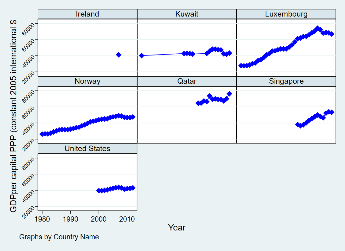
The first figure
The first figure
cd Lab2
use wdipol.dta, clear
describe
keep if inlist(country, "Ireland","Kuwait","Luxembourg","Norway","Qatar","Singapore","United States")
egen max_gdppc = max(gdppc) if country=="Ireland"
drop if country=="Ireland" & gdppc<max_gdppc
drop if (country=="Singapore" | country=="United States") & year<2000
sort country year
preserve
keep if country=="Kuwait"
sort year
scalar kuwait_first = gdppc[1]
restore
sort country year
replace gdppc = . if country=="Kuwait" & gdppc < kuwait_first & _n > 1
graph twoway (connected gdppc year, msymbol(diamond) mcolor(blue) lcolor(blue)), by(country, cols(3) compact note("Graphs by Country Name")) ytitle("GDPper capital PPP (constant 2005 international $") xtitle("Year") legend(off) yscale(range(40000 .))
. cd Lab2
Lab2
. use wdipol.dta, clear
. describe
Contains data from wdipol.dta
obs: 4,542
vars: 12 25 Feb 2015 17:31
size: 381,528
--------------------------------------------------------------------------------------------------
storage display value
variable name type format label variable label
--------------------------------------------------------------------------------------------------
year int %10.0g Year
country str24 %24s Country Name
gdppc double %10.0g GDP per capita, PPP (constant 2005 international $)
unempf double %10.0g Unemployment, female (% of female labor force)
unempm double %10.0g Unemployment, male (% of male labor force)
unemp double %10.0g Unemployment, total (% of total labor force)
export double %10.0g Exports of goods and services (constant 2005 US$)
import double %10.0g Imports of goods and services (constant 2005 US$)
polity byte %8.0g polity (original)
polity2 byte %8.0g polity2 (adjusted)
trade float %9.0g Imports + Exports
id float %9.0g group(country)
-------------------------------------------------------------------------------------------------
Sorted by:
. keep if inlist(country, "Ireland","Kuwait","Luxembourg","Norway","Qatar","Singapore","United States")
(4,358 observations deleted)
. egen max_gdppc = max(gdppc) if country=="Ireland"
(171 missing values generated)
. drop if country=="Ireland" & gdppc<max_gdppc
(12 observations deleted)
. drop if (country=="Singapore" | country=="United States") & year<2000
(40 observations deleted)
. sort country year
. preserve
. keep if country=="Kuwait"
(105 observations deleted)
. sort year
. scalar kuwait_first = gdppc[1]
. restore
. sort country year
. replace gdppc = . if country=="Kuwait" & gdppc < kuwait_first & _n > 1
(13 real changes made, 13 to missing)
. graph twoway (connected gdppc year, msymbol(diamond) mcolor(blue) lcolor(blue)), by(country, cols(3) compact note("Graphs by
> Country Name")) ytitle("GDPper capital PPP (constant 2005 international $") xtitle("Year") legend(off) yscale(range(40000 .
> ))Then you can use the graph editor to modify the layout.
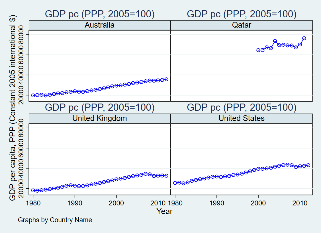
The second figure
The second figure
cd Lab2
use wdipol.dta, clearkeep if inlist(country, "Australia", "Qatar", "United Kingdom", "United States")
sort country year
graph twoway (connected gdppc year, msymbol(o) mcolor(blue) lcolor(blue)), by(country, rows(2) compact note("Graphs by Country Name")) title("GDP pc (PPP, 2005=100)") ytitle("GDP per capita, PPP (Constant 2005 international $)") xtitle("Year") legend(off)
. cd Lab2
Lab2
. use wdipol.dta, clear
. keep if inlist(country, "Australia", "Qatar", "United Kingdom", "United States")
(4,431 observations deleted)
. sort country year
. graph twoway (connected gdppc year, msymbol(o) mcolor(blue) lcolor(blue)), by(country, rows(2) compact note("Graphs by Count
> ry Name")) title("GDP pc (PPP, 2005=100)") ytitle("GDP per capita, PPP (Constant 2005 international $)") xtitle("Year") lege
> nd(off)Then you can use the graph editor to modify the layout.
Data Visualization in Econometrics
SLEEP75
Using the SLEEP75 data from Biddle and Hamermesh (1990), examine whether there is a trade-off between the time spent sleeping each week and the time spent on paid work. We can use either of these variables as the dependent variable.
1. Estimate the model: $$\text{sleep} = \beta_0 + \beta_1 \text{totwrk} + \mu$$
Where $\text{sleep}$ represents the number of minutes spent sleeping at night each week, and $\text{totwrk}$ represents the number of minutes spent on paid work during the same week. Report your results in equation form, along with the number of observations and $R^2$. What does the intercept in this equation represent?
cd Lab2
use SLEEP75.dta
describe sleep totwrk
reg sleep totwrk
. cd Lab2
Lab2
. use SLEEP75.dta
. describe sleep totwrk
storage display value
variable name type format label variable label
------------------------------------------------------------------------------------------------------------------------------
sleep int %9.0g mins sleep at night, per wk
totwrk int %9.0g mins worked per week
. reg sleep totwrk
Source | SS df MS Number of obs = 706
-------------+---------------------------------- F(1, 704) = 81.09
Model | 14381717.2 1 14381717.2 Prob > F = 0.0000
Residual | 124858119 704 177355.282 R-squared = 0.1033
-------------+---------------------------------- Adj R-squared = 0.1020
Total | 139239836 705 197503.313 Root MSE = 421.14
------------------------------------------------------------------------------
sleep | Coef. Std. Err. t P>|t| [95% Conf. Interval]
-------------+----------------------------------------------------------------
totwrk | -.1507458 .0167403 -9.00 0.000 -.1836126 -.117879
_cons | 3586.377 38.91243 92.17 0.000 3509.979 3662.775
------------------------------------------------------------------------------From the results above, we have the model: $$\text{sleep} = 3586.377 – 0.1507458 \cdot \text{totwrk} + \mu$$
The intercept $\beta_0$ represents the expected number of minutes of nightly sleep per week when $\text{totwrk}= 0$. In other words, it reflects the predicted total weekly nighttime sleep in the absence of paid work.
2. If $\text{totwrk}$ increases by 2 hours, by how much is $\text{sleep}$ estimated to decrease? Do you think this is a significant effect?
If $\text{totwrk}$ increases by 2 hours, or 120 minutes, the estimated decrease in $\text{sleep}$ is calculated as:$\Delta \text{sleep} = \beta_1 \times 120 = -0.1507458 \times 120 \approx -18 \text{ minutes}$.
An additional 2 hours of work per week results in only an 18-minute reduction in sleep, which is not particularly significant. From a weekly perspective, this is seemingly a relatively small impact.
WAGE2
Using data from WAGE2, estimate a simple regression to explain monthly wages using intelligence quotient.
1. Calculate the average (here, you can use mean value to represent the average value) wage and the average IQ in the sample. What is the sample standard deviation of IQ? (In the population, IQ is standardized with a mean of 100 and a standard deviation of 15.)
use WAGE2.dta, clear
summarize wage IQ
. use WAGE2.dta, clear
. summarize wage IQ
Variable | Obs Mean Std. Dev. Min Max
-------------+---------------------------------------------------------
wage | 935 957.9455 404.3608 115 3078
IQ | 935 101.2824 15.05264 50 145Mean wage : 957.9455
Mean IQ : 101.2824
Standard deviation of IQ : 15.05264
2. Estimate a simple regression model where an increase of one unit in IQ results in a specific change in wage. Using this model, calculate the expected change in wages when IQ increases by 15 units. Does IQ explain most of the variation in wages?
Here, we use Linear Model.
reg wage IQ. reg wage IQ
Source | SS df MS Number of obs = 935
-------------+---------------------------------- F(1, 933) = 98.55
Model | 14589782.6 1 14589782.6 Prob > F = 0.0000
Residual | 138126386 933 148045.429 R-squared = 0.0955
-------------+---------------------------------- Adj R-squared = 0.0946
Total | 152716168 934 163507.675 Root MSE = 384.77
------------------------------------------------------------------------------
wage | Coef. Std. Err. t P>|t| [95% Conf. Interval]
-------------+----------------------------------------------------------------
IQ | 8.303064 .8363951 9.93 0.000 6.661631 9.944498
_cons | 116.9916 85.64153 1.37 0.172 -51.08078 285.0639
------------------------------------------------------------------------------$$\text{wage} = 116.916 + 8.303064 \text{IQ}$$
An increase of 15 IQ points (approximately one standard deviation) would result in an estimated wage increase of $15 \times 8.303064 \approx 124.55$ USD per month.
$R^2 \approx 0.0955$ indicates that IQ explains less than 10% of the variation in wages. Most of the wage variation is determined by factors other than IQ.
3. Now estimate a model where an increase of one unit in IQ has the same percentage impact on wages. If IQ increases by 15 units, what is the approximate expected percentage increase in wages?
Here, we use Log-Linear Model.
reg lwage IQ. reg lwage IQ
Source | SS df MS Number of obs = 935
-------------+---------------------------------- F(1, 933) = 102.62
Model | 16.4150939 1 16.4150939 Prob > F = 0.0000
Residual | 149.241189 933 .159958402 R-squared = 0.0991
-------------+---------------------------------- Adj R-squared = 0.0981
Total | 165.656283 934 .177362188 Root MSE = .39995
------------------------------------------------------------------------------
lwage | Coef. Std. Err. t P>|t| [95% Conf. Interval]
-------------+----------------------------------------------------------------
IQ | .0088072 .0008694 10.13 0.000 .007101 .0105134
_cons | 5.886994 .0890206 66.13 0.000 5.712291 6.061698
------------------------------------------------------------------------------$$\ln(\text{wage}) = 5.887 + 0.0088072 \text{IQ}$$
An increase of 15 IQ points would lead to an estimated wage increase of $15 \times 0.88\% \approx 13.2\%$.
Lab 3
Macro
Use macro to draw a heart curve. We suggest you using the following curve:$$\begin{cases} x = \sin(t) \cos(t) \ln(|t|), \\ y = |t|^{0.3} \sqrt{\cos(t)}, \end{cases} \quad t \in \left[-\frac{\pi}{2}, \frac{\pi}{2}\right]$$
clear
set obs 50000
tempvar t
gen `t' = runiform(-0.5 * _pi, 0.5 * _pi)
sort `t'
local heart
local points = 50
local runs = 200
local i = 1
while `i' <= `runs' {
    display "`i'"
    tempvar control`i' x`i' y`i'
    gen `control`i'' = int(runiform(1,_N))
    gen `x`i'' = sin(`t')*cos(`t')*ln(abs(`t')) if `control`i'' <= `points'
    gen `y`i'' = (abs(`t'))^(0.3)*(cos(`t'))^(0.5) if `control`i'' <= `points'
    local heart `heart' (area `y`i'' `x`i'', nodropbase lc(black) lw(vthin) fc(red%5))
    local i = `i' + 1
}
twoway `heart', aspect(0.8) xscale(off) yscale(off) xlabel(, nogrid) ylabel(, nogrid) legend(off) xsize(1) ysize(1)
. clear
. set obs 50000
number of observations (_N) was 0, now 50,000
. tempvar t
. gen `t' = runiform(-0.5 * _pi, 0.5 * _pi)
. sort `t'
. local heart
. local points = 50
. local runs = 200
. local i = 1
. while `i' <= `runs' {
2. display "`i'"
3. tempvar control`i' x`i' y`i'
4. gen `control`i'' = int(runiform(1,_N))
5. gen `x`i'' = sin(`t')*cos(`t')*ln(abs(`t')) if `control`i'' <= `points'
6. gen `y`i'' = (abs(`t'))^(0.3)*(cos(`t'))^(0.5) if `control`i'' <= `points'
7. local heart `heart' (area `y`i'' `x`i'', nodropbase lc(black) lw(vthin) fc(red%5))
8. local i = `i' + 1
9. }
1
(49,943 missing values generated)
(49,943 missing values generated)
2
(49,949 missing values generated)
(49,949 missing values generated)
3
(49,945 missing values generated)
(49,945 missing values generated)
........................................................
200
(49,950 missing values generated)
(49,950 missing values generated)
. twoway `heart', aspect(0.8) xscale(off) yscale(off) xlabel(, nogrid) ylabel(, nogrid) legend(off) xsize(1) ysize(1)
Group Assignment
Requirements
- Use a
.dofile to collect all commands. - Data is from the paper Americans Do IT Better: US Multinationals and the Productivity Miracle by Nick Bloom, Rafaella Sadun, and John van Reenen, forthcoming in the American Economic Review.
- Submit as a group; only one submission per group is required.
- The submission format should be:
StudentID1+Name1+StudentID2+Name2.do, for example:202422+Amamitsu+202423+Yanagi.do. - Data and the paper are attached.
- At the beginning of the
.dofile, include comments listing the student ID and name of every group member. - Use comments to label each question with its corresponding number. (If a question number is missing, it will be treated as incomplete.)
- For questions requiring explanations, answer using comments.
- Ensure your
.dofile can execute correctly without errors.
Questions
1. Open the dataset replicate.dta.
cd Lab3
use replicate.dta, clear
The output:
. cd Lab3
Lab3

. use replicate.dta, clear
2. Use the describe command to determine the number of observations and identify the variable containing “people management” score information.
describeThe output:
. describe

Contains data from replicate.dta
  obs:         8,417
 vars:            33                          17 Oct 2011 19:33
 size:       942,704                          (_dta has notes)
--------------------------------------------------------------------------------------------------------------------------
              storage   display    value
variable name   type    format     label      variable label
--------------------------------------------------------------------------------------------------------------------------
analyst         str10   %10s                  Person that ran the interview
company_code    int     %9.0g                 Individual company level code - not the actual BVD number for anonymity
cover           float   %9.0g                 Share of employees in the firm surveyed by Harte-Hanks
cty             str2    %9s                   Country
du_oth_mu       byte    %9.0g                 Non-US multinational
du_usa_mu       byte    %9.0g                 US multinational
employees_a     int     %8.0g                 Firm level employees
hours_t         float   %9.0g                 Average works worked by employees
interview       int     %9.0g                 Code for each interview - ordered by company and interviewer
lcap            float   %9.0g                 Log(net tangible fixed assets) in current dollars per employee
ldegree_t       float   %9.0g                 Log(employees with a degree), with missing set to -99
ldegree_t_miss  byte    %9.0g                 Missing dummy for Log(employees with a degree)
lemp            float   %9.0g                 Log(employees in the firm)
lmat            float   %9.0g                 Log(materials) in current dollars
lpcemp          float   %9.0g                 Log of computers per employee, set to zero for missing values
lpcemp_du_oth~u float   %9.0g                 Interaction of log(pcemp) with non-US multinational ownership
lpcemp_du_usa~u float   %9.0g                 Interaction of log(pcemp) with US multinational ownership
lpcemp_ldegre~t float   %9.0g                 log(pcemp) interacted with log(degree)
lpcemp_ldegre~s float   %9.0g                 log(pcemp) interacted with log(degree)_miss
lpcemp_peeps    float   %9.0g                 Interaction of log(pcemp) with people management
ly              float   %9.0g                 Log(sales) in current dollars
management      float   %9.0g                 Average of all management practices z-scores, normalized to SD of 1
monitoring      float   %9.0g                 Average of monitoring management practices z-scores, normalized to SD of 1
operations      float   %9.0g                 Average of operations management practices z-scores, normalized to SD of 1
peeps           float   %9.0g                 Average of people management, normalized to SD of 1
public          byte    %8.0g      public     Publicly listed company, -99 for missing
publicmiss      byte    %9.0g                 Publicly listed company missing dummy
s_count         byte    %9.0g                 1=Unique match of HH site to BVD code. 0=Multiple matches or jumps, .=no match
sic             int     %8.0g                 US Sic code
targets         float   %9.0g                 Average of targets management practices z-scores, normalized to SD of 1
union           float   %8.0g                 Pct of union members
wages_a         double  %8.0g                 Cost of employees, 000$
year            int     %9.0g                 year of the accounts and IT data (all management data collected in 2006)
--------------------------------------------------------------------------------------------------------------------------
Sorted by: interview  year
From the description, we know that peeps holds the information of people management, the corresponding log value is lpcemp_peeps.
3. Find the mean of the “people management” score.
summarize peeps, detailThe output:
. summarize peeps, detail

      Average of people management, normalized to SD of
                              1
-------------------------------------------------------------
      Percentiles      Smallest
 1%    -1.464864      -1.693648
 5%    -1.214176      -1.693648
10%    -.9772028      -1.693648       Obs               8,417
25%    -.5124432      -1.693648       Sum of Wgt.       8,417

50%    -.0391659                      Mean          -.0192126
                        Largest       Std. Dev.      .7060643
75%      .433783       2.087268
90%      .906063       2.087268       Variance       .4985268
95%     1.148562       2.087268       Skewness       .1634675
99%     1.621511       2.087268       Kurtosis       2.699202
The mean value is -0.0192.
4. Use the tabulate command to identify the countries and years in the sample, and the number of observations for each year and country.
tabulate cty year, missingThe output:
. tabulate cty year, missing

           |        year of the accounts and IT data (all management data collected in 2006)
   Country |      1999       2000       2001       2002       2003       2004       2005       2006 |     Total
-----------+----------------------------------------------------------------------------------------+----------
        fr |       189        166        191        216        218        232        232          8 |     1,452
        ge |        59         57         61         72         82         83         59          1 |       474
        it |        97        130        141        149        137        155        106          3 |       918
        po |        70         87        102        172        167        166         86          0 |       850
        pt |        48         46         52         79        120        101         57          0 |       503
        sw |       167        179        125        175        179        199        183          6 |     1,213
        uk |       327        422        413        454        457        479        425         30 |     3,007
-----------+----------------------------------------------------------------------------------------+----------
     Total |       957      1,087      1,085      1,317      1,360      1,415      1,148         48 |     8,417
5. What are the mean, standard deviation, and number of observations for employment levels in UK companies? Calculate these statistics separately for US multinationals, other multinationals, and UK domestic firms to replicate column 1 of Table 1.
gen byte company_type = .
replace company_type = 1 if du_usa_mu == 1
replace company_type = 2 if du_oth_mu == 1
replace company_type = 3 if du_usa_mu == 0 & du_oth_mu == 0
label define company_type_lbl 1 "US Multinational" 2 "Non-US Multinational" 3 "UK Domestic"
label values company_type company_type_lbl
tabulate company_type
tabstat employees_a, by(company_type) statistics(mean sd count) columns(statistics)
The output:
. gen byte company_type = .
(8,417 missing values generated)

. replace company_type = 1 if du_usa_mu == 1
(919 real changes made)

. replace company_type = 2 if du_oth_mu == 1
(2,172 real changes made)

. replace company_type = 3 if du_usa_mu == 0 & du_oth_mu == 0
(5,326 real changes made)

. label define company_type_lbl 1 "US Multinational" 2 "Non-US Multinational" 3 "UK Domestic"

. label values company_type company_type_lbl

. tabulate company_type

        company_type |      Freq.     Percent        Cum.
---------------------+-----------------------------------
    US Multinational |        919       10.92       10.92
Non-US Multinational |      2,172       25.80       36.72
         UK Domestic |      5,326       63.28      100.00
---------------------+-----------------------------------
               Total |      8,417      100.00

. tabstat employees_a, by(company_type) statistics(mean sd count) columns(statistics)

Summary for variables: employees_a
     by categories of: company_type

    company_type |      mean        sd         N
-----------------+------------------------------
US Multinational |  495.2688  645.1402       919
Non-US Multinati |   428.785  509.3583      2172
     UK Domestic |  417.6536   650.362      5326
-----------------+------------------------------
           Total |  429.0004  616.8552      8417
------------------------------------------------
6. Find the average management score for each country and year.
preserve
collapse (mean) avg_management=management, by(cty year)
list
restore
The output:
. preserve

. collapse (mean) avg_management=management, by(cty year)

. list

     +------------------------+
     | cty   year   avg_man~t |
     |------------------------|
  1. |  fr   1999    .0334847 |
  2. |  fr   2000    .0048502 |
  3. |  fr   2001    .0730181 |
  4. |  fr   2002    .0875922 |
  5. |  fr   2003    .0530531 |
     |------------------------|
  6. |  fr   2004    .0823055 |
  7. |  fr   2005    .1030681 |
  8. |  fr   2006   -.0640106 |
  9. |  ge   1999    .4130789 |
 10. |  ge   2000    .3726625 |
     |------------------------|
 11. |  ge   2001    .4496971 |
 12. |  ge   2002    .3818938 |
 13. |  ge   2003    .4633776 |
 14. |  ge   2004    .4582495 |
 15. |  ge   2005    .4307467 |
     |------------------------|
 16. |  ge   2006    .6042405 |
 17. |  it   1999    .0388724 |
 18. |  it   2000    .0418419 |
 19. |  it   2001    .0179532 |
 20. |  it   2002    .0626969 |
     |------------------------|
 21. |  it   2003    .0075816 |
 22. |  it   2004    .0139907 |
 23. |  it   2005    .0230397 |
 24. |  it   2006     .661514 |
 25. |  po   1999   -.0150875 |
     |------------------------|
 26. |  po   2000    .1379714 |
 27. |  po   2001      .08615 |
 28. |  po   2002    .0266212 |
 29. |  po   2003   -.1027957 |
 30. |  po   2004   -.0598225 |
     |------------------------|
 31. |  po   2005   -.0460614 |
 32. |  pt   1999   -.1548034 |
 33. |  pt   2000   -.1954222 |
 34. |  pt   2001   -.3220826 |
 35. |  pt   2002   -.3969625 |
     |------------------------|
 36. |  pt   2003   -.3443317 |
 37. |  pt   2004   -.3615427 |
 38. |  pt   2005   -.5732161 |
 39. |  sw   1999    .3488918 |
 40. |  sw   2000    .3164622 |
     |------------------------|
 41. |  sw   2001    .3725764 |
 42. |  sw   2002     .336567 |
 43. |  sw   2003    .2955157 |
 44. |  sw   2004    .3070801 |
 45. |  sw   2005    .2999685 |
     |------------------------|
 46. |  sw   2006   -.4343244 |
 47. |  uk   1999    .0758213 |
 48. |  uk   2000    .0747772 |
 49. |  uk   2001    .1105612 |
 50. |  uk   2002    .0898244 |
     |------------------------|
 51. |  uk   2003    .0839255 |
 52. |  uk   2004     .069181 |
 53. |  uk   2005    .0531464 |
 54. |  uk   2006   -.0244585 |
     +------------------------+

. restore
7. Create a horizontal bar chart showing the average “people management” score for each country, replicating Figure 3a from the paper.
preserve
collapse (mean) avg_peeps=peeps, by(cty)
gen sort_order = -avg_peeps
graph hbar avg_peeps, over(cty, sort(sort_order)) title("Average People Management Scores by Country") ylabel(, angle(0)) scheme(s1color)
graph export "Average_People_Management_by_Country.png", width(800) replace
restore
The output:
. preserve

. collapse (mean) avg_peeps=peeps, by(cty)

. gen sort_order = -avg_peeps

. graph hbar avg_peeps, over(cty, sort(sort_order)) title("Average People Manag
> ement Scores by Country") ylabel(, angle(0)) scheme(s1color)

. graph export "Average_People_Management_by_Country.png", width(800) replace
(file Average_People_Management_by_Country.png written in PNG format)

. restore
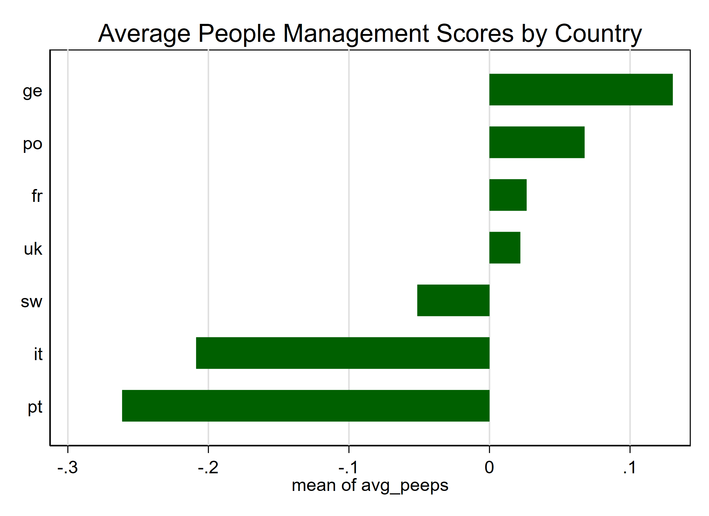
8. Repeat the same chart but include only US multinational subsidiaries.
preserve
keep if company_type == 1
collapse (mean) avg_peeps=peeps, by(cty)
gen sort_order = -avg_peeps
graph hbar avg_peeps, over(cty, sort(sort_order)) title("Average People Management Scores by Country (US Multinationals)") ylabel(, angle(0)) scheme(s1color)
graph export "Average_People_Management_US_Multinationals.png", width(800) replace
restore
The output:
. preserve

. keep if company_type == 1
(7,498 observations deleted)

. collapse (mean) avg_peeps=peeps, by(cty)

. gen sort_order = -avg_peeps

. graph hbar avg_peeps, over(cty, sort(sort_order)) title("Average People Manag
> ement Scores by Country (US Multinationals)") ylabel(, angle(0)) scheme(s1col
> or)

.
. graph export "Average_People_Management_US_Multinationals.png", width(800) re
> place
(file Average_People_Management_US_Multinationals.png written in PNG format)

.
. restore
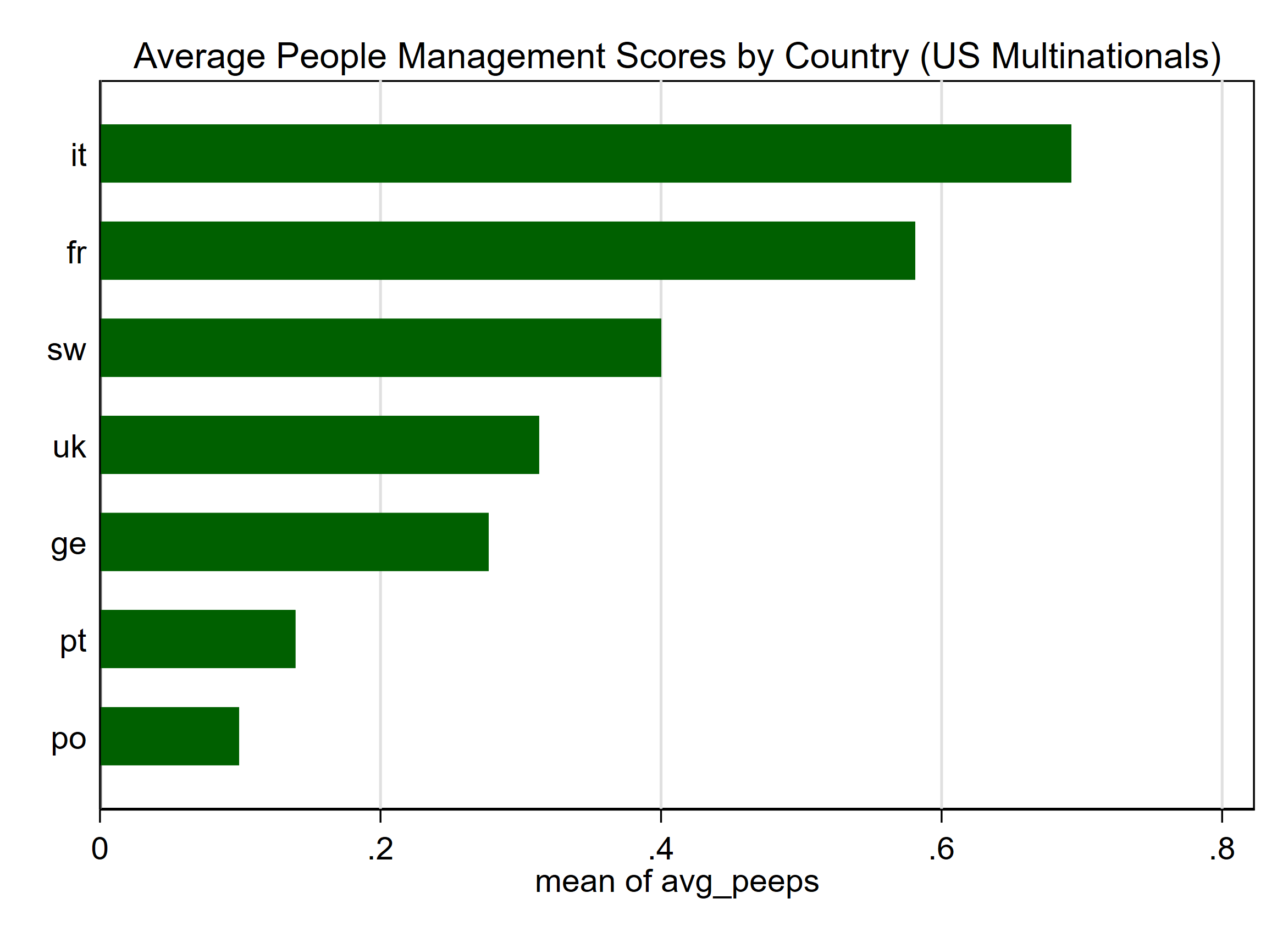
9. Generate a variable equal to the total working hours of the company.
gen total_hours = employees_a * hours_tThe output:
. gen total_hours = employees_a * hours_t
(725 missing values generated)
10. List the top 10 observations to verify whether your new variable is correctly defined.
list company_code cty year employees_a hours_t total_hours in 1/10The output:
. list company_code cty year employees_a hours_t total_hours in 1/10

     +-------------------------------------------------------+
     | compa~de   cty   year   employ~a   hours_t   total_~s |
     |-------------------------------------------------------|
  1. |        3    ge   2001        465      4176    1941840 |
  2. |        3    ge   2002        526      4176    2196576 |
  3. |        4    ge   2001       2113      3920    8282960 |
  4. |        4    ge   2002       1996      3920    7824320 |
  5. |        4    ge   2003       1853      3920    7263760 |
     |-------------------------------------------------------|
  6. |        4    ge   2004       1888      3920    7400960 |
  7. |        5    ge   2001       2261         .          . |
  8. |        5    ge   2002       2273         .          . |
  9. |        5    ge   2003       2336         .          . |
 10. |        5    ge   2004       2518         .          . |
     +-------------------------------------------------------+
10+. Drop the variable you defined just before
drop total_hoursThe output:
. drop total_hours
11. Create a dummy variable (0/1) where the value is 1 if the company has at least one union member and 0 otherwise. (Hint: Use generate, replace, and if together.)
generate union_dummy = 0
replace union_dummy = 1 if union > 0
The output:
. generate union_dummy = 0

. replace union_dummy = 1 if union > 0
(6,294 real changes made)
12. Rename the management score variable to start with a common prefix, such as m_peeps.
rename peeps m_peepsThe output:
. rename peeps m_peeps
13. Create a variable representing the total sum of all individual management scores. Compare this to the existing variable management. Why are they different? Explain the discrepancy and adjust the formula until the two variables match.
This result is still not correct. But the teacher said it is okay.
drop if missing(m_peeps, monitoring, operations, targets)
foreach var of varlist m_peeps monitoring operations targets {
    summarize `var'
    scalar mean_`var' = r(mean)
    scalar sd_`var'   = r(sd)
    gen double `var'_z2 = (`var' - mean_`var') / sd_`var'
}
egen management_sum_avg2 = rowmean(m_peeps_z2 monitoring_z2 operations_z2 targets_z2)
summarize management_sum_avg2
scalar mean_m2 = r(mean)
scalar sd_m2   = r(sd)
gen management_sum_z2 = (management_sum_avg2 - mean_m2) / sd_m2
summarize management_sum_z2 management
correlate management_sum_z2 management
The output:
.  drop if missing(m_peeps, monitoring, operations, targets)
(7 observations deleted)

. foreach var of varlist m_peeps monitoring operations targets {
  2.
.     summarize `var'
  3.
.     scalar mean_`var' = r(mean)
  4.
.     scalar sd_`var'   = r(sd)
  5.
.     gen double `var'_z2 = (`var' - mean_`var') / sd_`var'
  6.
. }

    Variable |        Obs        Mean    Std. Dev.       Min        Max
-------------+---------------------------------------------------------
     m_peeps |      8,410   -.0188083     .706219  -1.693648   2.087268

    Variable |        Obs        Mean    Std. Dev.       Min        Max
-------------+---------------------------------------------------------
  monitoring |      8,410    .0671427    1.008082  -2.976081   2.434706

    Variable |        Obs        Mean    Std. Dev.       Min        Max
-------------+---------------------------------------------------------
  operations |      8,410     .138289    1.011542   -2.05452   2.352676

    Variable |        Obs        Mean    Std. Dev.       Min        Max
-------------+---------------------------------------------------------
     targets |      8,410    .1176681    1.012729  -2.619704   2.805768

. egen management_sum_avg2 = rowmean(m_peeps_z2 monitoring_z2 operations_z2 targets_z2)

. summarize management_sum_avg2

    Variable |        Obs        Mean    Std. Dev.       Min        Max
-------------+---------------------------------------------------------
management~2 |      8,410    3.35e-10    .8171414  -2.406625   2.252212

. scalar mean_m2 = r(mean)

. scalar sd_m2   = r(sd)

. gen management_sum_z2 = (management_sum_avg2 - mean_m2) / sd_m2

. summarize management_sum_z2 management

    Variable |        Obs        Mean    Std. Dev.       Min        Max
-------------+---------------------------------------------------------
managemen~z2 |      8,410   -1.81e-11           1  -2.945175   2.756208
  management |      8,410    .0921417    1.012059  -3.019884   2.841167

. correlate management_sum_z2 management
(obs=8,410)

             | manag~z2 manage~t
-------------+------------------
managemen~z2 |   1.0000
  management |   0.9872   1.0000

. scatter management_sum_z2 management

. correlate management_sum_avg2 management
(obs=8,410)

             | manag~g2 manage~t
-------------+------------------
managemen~g2 |   1.0000
  management |   0.9872   1.0000
14. Perform a regression analysis of log(sales) on log(employees in the firm).
regress ly lempThe output:
. regress ly lemp

      Source |       SS           df       MS      Number of obs   =     8,417
-------------+----------------------------------   F(1, 8415)      =     26.46
       Model |  16.4187464         1  16.4187464   Prob > F        =    0.0000
    Residual |  5221.37628     8,415  .620484407   R-squared       =    0.0031
-------------+----------------------------------   Adj R-squared   =    0.0030
       Total |  5237.79503     8,416  .622361577   Root MSE        =    .78771

------------------------------------------------------------------------------
          ly |      Coef.   Std. Err.      t    P>|t|     [95% Conf. Interval]
-------------+----------------------------------------------------------------
        lemp |   .0495207   .0096268     5.14   0.000     .0306498    .0683916
       _cons |   4.822661   .0545029    88.48   0.000     4.715822      4.9295
------------------------------------------------------------------------------
15. Predict fitted values and create a chart plotting a scatterplot of log(sales) against log(employees in the firm) with a fitted line.
predict fitted_ly
twoway (scatter ly lemp) (line fitted_ly lemp), title("Log(Sales) vs Log(Employees) with Fit Line")  legend(order(1 "Actual" 2 "Fitted")) xlabel(, angle(vertical)) ylabel(, angle(horizontal)) scheme(s1color)
graph export "LogSales_vs_LogEmployees_with_FitLine.png", width(800) replace
The output:
. predict fitted_ly
(option xb assumed; fitted values)

. twoway (scatter ly lemp) (line fitted_ly lemp), title("Log(Sales) vs Log(Employees) with Fit Line")  legend(order(1 "Actual" 2 "Fitted")) xlabel(, angl
> e(vertical)) ylabel(, angle(horizontal)) scheme(s1color)

. graph export "LogSales_vs_LogEmployees_with_FitLine.png", width(800) replace
(file LogSales_vs_LogEmployees_with_FitLine.png written in PNG format)
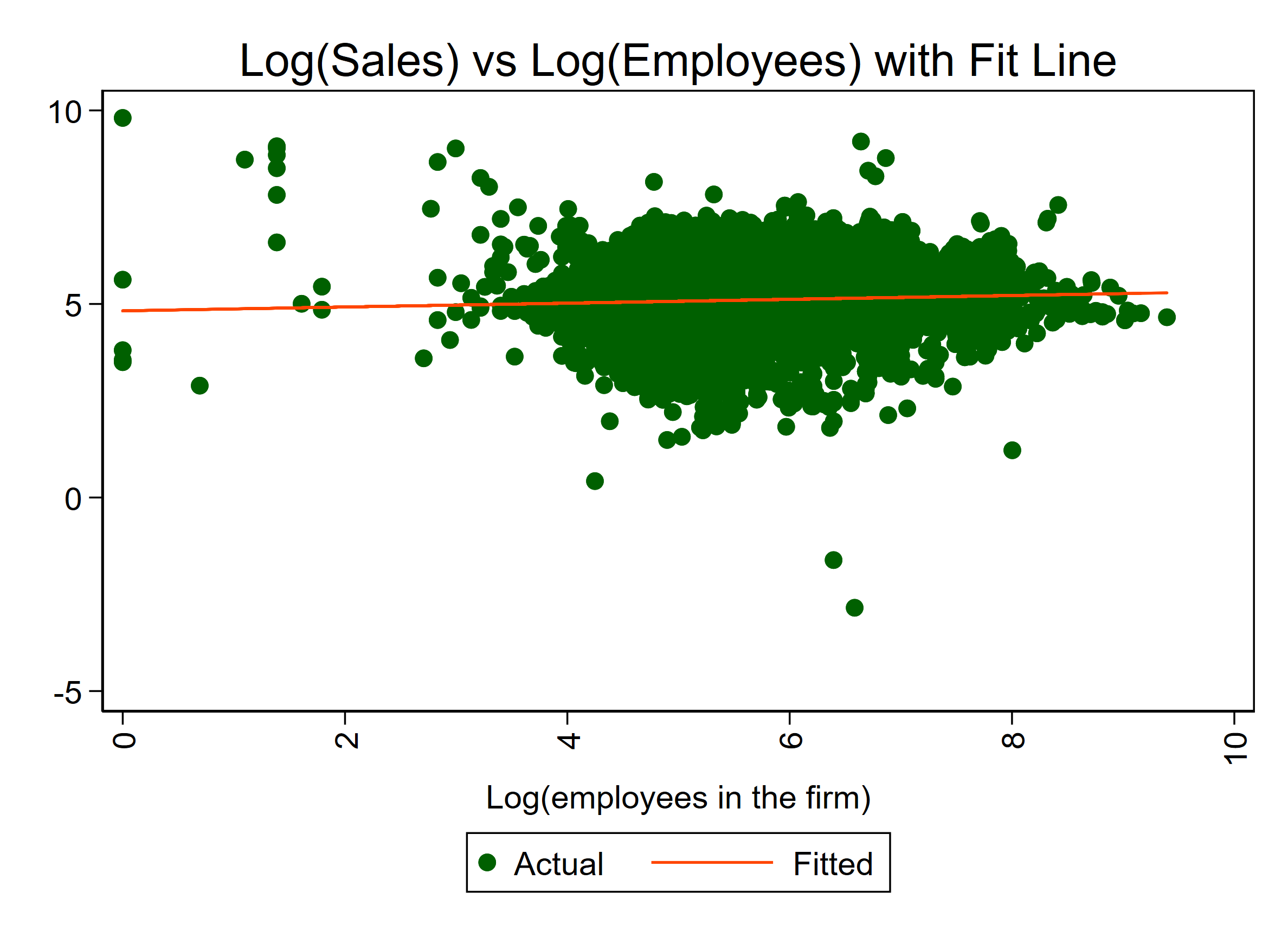
16. Repeat the same regression, but this time limit the sample to:
i) UK domestic companies,
ii) US multinational companies,
iii) other multinational companies.
Plot three separate fitted lines on the scatterplot.
regress ly lemp if company_type == 3
predict fitted_uk if company_type == 3
regress ly lemp if company_type == 1
predict fitted_us if company_type == 1
regress ly lemp if company_type == 2
predict fitted_oth if company_type == 2
twoway (scatter ly lemp if company_type == 3, mcolor(eltblue) msymbol(Oh) msize(small) legend(label(1 "UK Domestic (scatter)")))(line fitted_uk lemp if company_type == 3, lcolor(blue) lwidth(medium) legend(label(2 "UK Domestic (line)")))(scatter ly lemp if company_type == 1, mcolor(pink) msymbol(Oh) msize(small) legend(label(3 "US Multinational (scatter)")))(line fitted_us lemp if company_type == 1, lcolor(red) lwidth(medium) legend(label(4 "US Multinational (line)")))(scatter ly lemp if company_type == 2, mcolor(olive_teal) msymbol(Oh) msize(small) legend(label(5 "Other Multinational (scatter)")))(line fitted_oth lemp if company_type == 2, lcolor(lime) lwidth(medium) legend(label(6 "Other Multinational (line)"))),title("Log(sales) vs. Log(employees) by Company Type") xtitle("Log(employees in the firm)") ytitle("Log(sales)") legend(order(1 2 3 4 5 6) region(style(none)) position(6) col(2) size(small))
The output:
. regress ly lemp if company_type == 3

      Source |       SS           df       MS      Number of obs   =     5,326
-------------+----------------------------------   F(1, 5324)      =     13.36
       Model |  8.28050094         1  8.28050094   Prob > F        =    0.0003
    Residual |  3299.94842     5,324  .619825023   R-squared       =    0.0025
-------------+----------------------------------   Adj R-squared   =    0.0023
       Total |  3308.22892     5,325  .621263648   Root MSE        =    .78729

------------------------------------------------------------------------------
          ly |      Coef.   Std. Err.      t    P>|t|     [95% Conf. Interval]
-------------+----------------------------------------------------------------
        lemp |   .0436063   .0119304     3.66   0.000     .0202178    .0669948
       _cons |   4.742818   .0669286    70.86   0.000      4.61161    4.874025
------------------------------------------------------------------------------

.
. predict fitted_uk if company_type == 3
(option xb assumed; fitted values)
(3,091 missing values generated)

.
. regress ly lemp if company_type == 1

      Source |       SS           df       MS      Number of obs   =       919
-------------+----------------------------------   F(1, 917)       =     16.89
       Model |  8.24884946         1  8.24884946   Prob > F        =    0.0000
    Residual |  447.783833       917  .488313885   R-squared       =    0.0181
-------------+----------------------------------   Adj R-squared   =    0.0170
       Total |  456.032682       918  .496767628   Root MSE        =    .69879

------------------------------------------------------------------------------
          ly |      Coef.   Std. Err.      t    P>|t|     [95% Conf. Interval]
-------------+----------------------------------------------------------------
        lemp |   -.105811   .0257444    -4.11   0.000    -.1563359   -.0552861
       _cons |   5.963486   .1497717    39.82   0.000     5.669551    6.257421
------------------------------------------------------------------------------

.
. predict fitted_us if company_type == 1
(option xb assumed; fitted values)
(7,498 missing values generated)

.
. regress ly lemp if company_type == 2

      Source |       SS           df       MS      Number of obs   =     2,172
-------------+----------------------------------   F(1, 2170)      =     16.94
       Model |  9.88791441         1  9.88791441   Prob > F        =    0.0000
    Residual |  1266.64783     2,170  .583708676   R-squared       =    0.0077
-------------+----------------------------------   Adj R-squared   =    0.0073
       Total |  1276.53574     2,171  .587994353   Root MSE        =    .76401

------------------------------------------------------------------------------
          ly |      Coef.   Std. Err.      t    P>|t|     [95% Conf. Interval]
-------------+----------------------------------------------------------------
        lemp |   .0797256   .0193706     4.12   0.000     .0417387    .1177124
       _cons |   4.822956   .1108085    43.53   0.000     4.605654    5.040258
------------------------------------------------------------------------------

.
. predict fitted_oth if company_type == 2
(option xb assumed; fitted values)
(6,245 missing values generated)

.
. twoway (scatter ly lemp if company_type == 3, mcolor(eltblue) msymbol(Oh) msize(small) legend(label(1 "UK Domestic (scatter)"
> )))(line fitted_uk lemp if company_type == 3, lcolor(blue) lwidth(medium) legend(label(2 "UK Domestic (line)")))(scatter ly l
> emp if company_type == 1, mcolor(pink) msymbol(Oh) msize(small) legend(label(3 "US Multinational (scatter)")))(line fitted_us
>  lemp if company_type == 1, lcolor(red) lwidth(medium) legend(label(4 "US Multinational (line)")))(scatter ly lemp if company
> _type == 2, mcolor(olive_teal) msymbol(Oh) msize(small) legend(label(5 "Other Multinational (scatter)")))(line fitted_oth lem
> p if company_type == 2, lcolor(lime) lwidth(medium) legend(label(6 "Other Multinational (line)"))),title("Log(sales) vs. Log(
> employees) by Company Type") xtitle("Log(employees in the firm)") ytitle("Log(sales)") legend(order(1 2 3 4 5 6) region(style
> (none)) position(6) col(2) size(small))
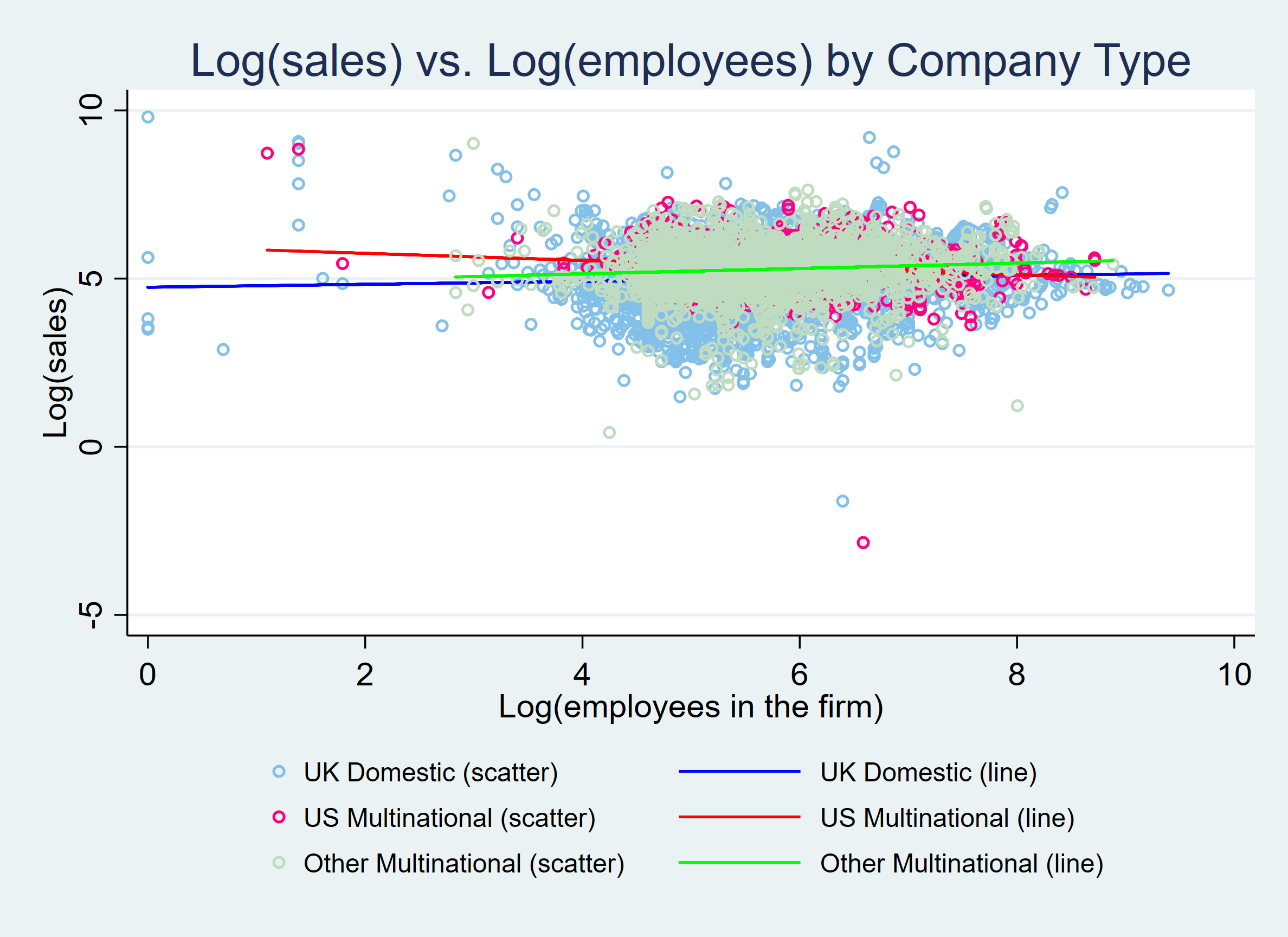
17. Rank companies based on year, country, and management score.
bysort year cty (management): gen rank = _N - _n +1
list company_code cty year management rank in 1/10
The output:
. bysort year cty (management): gen rank = _N - _n +1

. list company_code cty year management rank in 1/10

     +------------------------------------------+
     | compa~de   cty   year   managem~t   rank |
     |------------------------------------------|
  1. |      207    fr   1999     -2.2934    189 |
  2. |      237    fr   1999   -2.289897    188 |
  3. |      241    fr   1999   -2.118449    187 |
  4. |      140    fr   1999   -2.019981    186 |
  5. |      313    fr   1999   -1.942747    185 |
     |------------------------------------------|
  6. |      398    fr   1999   -1.869219    184 |
  7. |      158    fr   1999   -1.860743    183 |
  8. |      389    fr   1999   -1.835789    182 |
  9. |      402    fr   1999   -1.780855    181 |
 10. |      338    fr   1999   -1.761644    180 |
     +------------------------------------------+
17+. Generate a variable nobs to represent the number of observations for each company.
bysort company_code: egen nobs = count(company_code)The output:
. bysort company_code: egen nobs = count(company_code)
17++. Create a scatter plot of management scores and sales using only 10% of the observations for each country and year (randomly selected observations).
sort cty year
set seed 12345
by cty year: gen double rnd = runiform()
gen byte pick = (rnd < 0.1)
twoway (scatter management ly if pick == 1)
The output:
. sort cty year

. set seed 12345

. by cty year: gen double rnd = runiform()

. gen byte pick = (rnd < 0.1)

. twoway (scatter management ly if pick == 1)
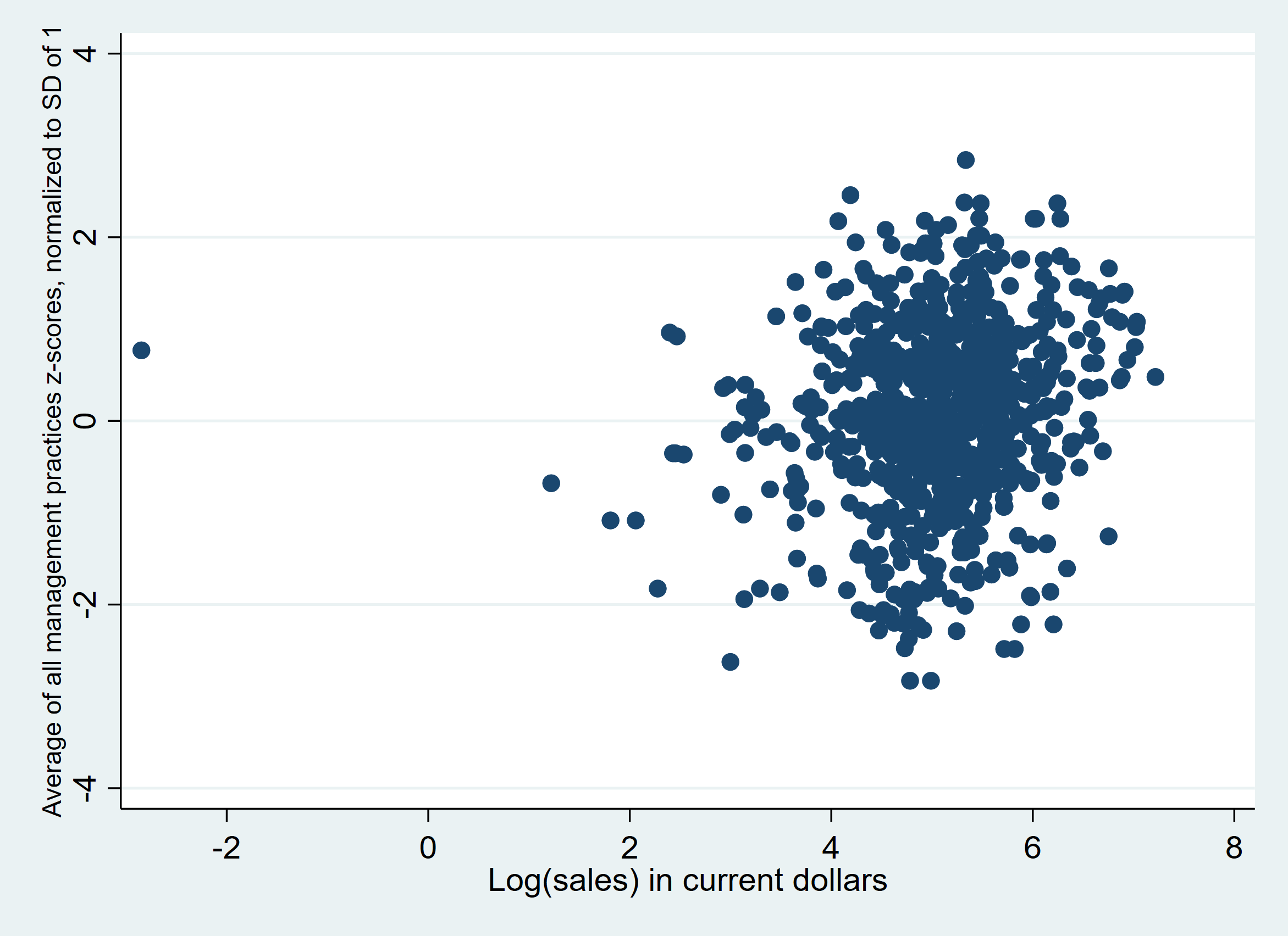
18. Regress log(sales) on log(materials), log(employment), and log(capital).
regress ly lmat lemp lcapThe output:
. regress ly lmat lemp lcap

      Source |       SS           df       MS      Number of obs   =     4,227
-------------+----------------------------------   F(3, 4223)      =   4983.44
       Model |  2315.18686         3  771.728954   Prob > F        =    0.0000
    Residual |  653.968595     4,223  .154858772   R-squared       =    0.7797
-------------+----------------------------------   Adj R-squared   =    0.7796
       Total |  2969.15546     4,226  .702592394   Root MSE        =    .39352

------------------------------------------------------------------------------
          ly |      Coef.   Std. Err.      t    P>|t|     [95% Conf. Interval]
-------------+----------------------------------------------------------------
        lmat |   .6332863   .0062647   101.09   0.000     .6210043    .6455683
        lemp |   .0013348   .0067869     0.20   0.844     -.011971    .0146407
        lcap |   .1230179   .0063333    19.42   0.000     .1106013    .1354345
       _cons |   2.025731   .0445252    45.50   0.000     1.938438    2.113024
------------------------------------------------------------------------------
19. Predict residuals and replace them with their squared values.
cd Lab3
use replicate.dta, clear
The output:
. predict residuals, residuals
(4,190 missing values generated)

. gen residuals_sq = residuals^2
(4,190 missing values generated)
20. Perform a regression of log(sales) on log(materials), log(employment), log(capital), and management for each country in the sample (use a loop).
levelsof cty, local(countries)
foreach country of local countries {
    display "Running regression for country: `country'"
    count if cty == "`country'" & !missing(ly, lmat, lemp, lcap, management)
    if r(N) > 0 regress ly lmat lemp lcap management if cty == "`country'"
    else display "Skipping country: `country' (insufficient non-missing observations)"
}
The output:
. levelsof cty, local(countries)
`"fr"' `"ge"' `"it"' `"po"' `"pt"' `"sw"' `"uk"'

. foreach country of local countries {
  2.
.     display "Running regression for country: `country'"
  3.
.     count if cty == "`country'" & !missing(ly, lmat, lemp, lcap, management)
  4.
.     if r(N) > 0 regress ly lmat lemp lcap management if cty == "`country'"
  5.
.     else display "Skipping country: `country' (insufficient non-missing observations)"
  6.
. }
Running regression for country: fr
  1,426

      Source |       SS           df       MS      Number of obs   =     1,426
-------------+----------------------------------   F(4, 1421)      =    756.57
       Model |  405.686127         4  101.421532   Prob > F        =    0.0000
    Residual |   190.49255     1,421  .134055278   R-squared       =    0.6805
-------------+----------------------------------   Adj R-squared   =    0.6796
       Total |  596.178678     1,425  .418371002   Root MSE        =    .36614

------------------------------------------------------------------------------
          ly |      Coef.   Std. Err.      t    P>|t|     [95% Conf. Interval]
-------------+----------------------------------------------------------------
        lmat |   .5123901    .011429    44.83   0.000     .4899707    .5348096
        lemp |   .0229771   .0131041     1.75   0.080    -.0027284    .0486826
        lcap |   .1112761   .0109944    10.12   0.000      .089709    .1328432
  management |   .0304229   .0109067     2.79   0.005      .009028    .0518178
       _cons |   2.634434   .0884672    29.78   0.000     2.460894    2.807975
------------------------------------------------------------------------------
Running regression for country: ge
  375

      Source |       SS           df       MS      Number of obs   =       375
-------------+----------------------------------   F(4, 370)       =    394.90
       Model |  96.6379666         4  24.1594916   Prob > F        =    0.0000
    Residual |  22.6362051       370  .061178933   R-squared       =    0.8102
-------------+----------------------------------   Adj R-squared   =    0.8082
       Total |  119.274172       374  .318914898   Root MSE        =    .24734

------------------------------------------------------------------------------
          ly |      Coef.   Std. Err.      t    P>|t|     [95% Conf. Interval]
-------------+----------------------------------------------------------------
        lmat |   .5343757   .0154031    34.69   0.000     .5040871    .5646644
        lemp |  -.0816476   .0137308    -5.95   0.000    -.1086478   -.0546474
        lcap |   .1213607   .0150875     8.04   0.000     .0916927    .1510286
  management |   .0246979    .015515     1.59   0.112    -.0058106    .0552065
       _cons |   3.044236   .1334112    22.82   0.000     2.781897    3.306575
------------------------------------------------------------------------------
Running regression for country: it
  905

      Source |       SS           df       MS      Number of obs   =       905
-------------+----------------------------------   F(4, 900)       =   1025.79
       Model |  268.180953         4  67.0452382   Prob > F        =    0.0000
    Residual |  58.8238441       900  .065359827   R-squared       =    0.8201
-------------+----------------------------------   Adj R-squared   =    0.8193
       Total |  327.004797       904   .36173097   Root MSE        =    .25566

------------------------------------------------------------------------------
          ly |      Coef.   Std. Err.      t    P>|t|     [95% Conf. Interval]
-------------+----------------------------------------------------------------
        lmat |   .5709453   .0104092    54.85   0.000     .5505162    .5913744
        lemp |    -.07023   .0105837    -6.64   0.000    -.0910016   -.0494584
        lcap |   .0976345   .0096953    10.07   0.000     .0786065    .1166625
  management |   .0267954   .0082875     3.23   0.001     .0105304    .0430603
       _cons |   2.802493   .0753308    37.20   0.000     2.654648    2.950337
------------------------------------------------------------------------------
Running regression for country: po
  562

      Source |       SS           df       MS      Number of obs   =       562
-------------+----------------------------------   F(4, 557)       =    423.87
       Model |  374.045352         4  93.5113379   Prob > F        =    0.0000
    Residual |  122.882657       557  .220615183   R-squared       =    0.7527
-------------+----------------------------------   Adj R-squared   =    0.7509
       Total |  496.928009       561  .885789676   Root MSE        =     .4697

------------------------------------------------------------------------------
          ly |      Coef.   Std. Err.      t    P>|t|     [95% Conf. Interval]
-------------+----------------------------------------------------------------
        lmat |   .4788854   .0185862    25.77   0.000     .4423779     .515393
        lemp |  -.1240909   .0253473    -4.90   0.000    -.1738788    -.074303
        lcap |   .2397321   .0206813    11.59   0.000     .1991092    .2803549
  management |   .0801802    .021518     3.73   0.000     .0379138    .1224466
       _cons |   2.534757   .1582044    16.02   0.000     2.224007    2.845507
------------------------------------------------------------------------------
Running regression for country: pt
  463

      Source |       SS           df       MS      Number of obs   =       463
-------------+----------------------------------   F(4, 458)       =    468.44
       Model |  218.307087         4  54.5767718   Prob > F        =    0.0000
    Residual |  53.3608483       458  .116508402   R-squared       =    0.8036
-------------+----------------------------------   Adj R-squared   =    0.8019
       Total |  271.667936       462  .588025835   Root MSE        =    .34133

------------------------------------------------------------------------------
          ly |      Coef.   Std. Err.      t    P>|t|     [95% Conf. Interval]
-------------+----------------------------------------------------------------
        lmat |   .6016575   .0177263    33.94   0.000     .5668226    .6364924
        lemp |  -.0094647   .0200062    -0.47   0.636      -.04878    .0298507
        lcap |   .1247086   .0198622     6.28   0.000     .0856763    .1637409
  management |   .0672758   .0167721     4.01   0.000     .0343161    .1002356
       _cons |   2.057761   .1312337    15.68   0.000     1.799866    2.315656
------------------------------------------------------------------------------
Running regression for country: sw
  496

      Source |       SS           df       MS      Number of obs   =       496
-------------+----------------------------------   F(4, 491)       =    603.13
       Model |   148.60951         4  37.1523775   Prob > F        =    0.0000
    Residual |  30.2451752       491  .061599135   R-squared       =    0.8309
-------------+----------------------------------   Adj R-squared   =    0.8295
       Total |  178.854685       495  .361322596   Root MSE        =    .24819

------------------------------------------------------------------------------
          ly |      Coef.   Std. Err.      t    P>|t|     [95% Conf. Interval]
-------------+----------------------------------------------------------------
        lmat |   .6121036   .0158239    38.68   0.000     .5810127    .6431945
        lemp |   .0455529   .0138143     3.30   0.001     .0184105    .0726953
        lcap |    .111258   .0121415     9.16   0.000     .0874024    .1351137
  management |  -.0211386   .0127182    -1.66   0.097    -.0461275    .0038502
       _cons |   1.941344   .0867648    22.37   0.000     1.770868     2.11182
------------------------------------------------------------------------------
Running regression for country: uk
  0
Skipping country: uk (insufficient non-missing observations)
20+. Test whether the coefficient of management is equal to 0.03 if it is statistically significant. If it is not significant, test whether it equals 0.03.
reg ly management
test _b[management] = 0.03
The output:
. reg ly management

      Source |       SS           df       MS      Number of obs   =     8,417
-------------+----------------------------------   F(1, 8415)      =    341.64
       Model |  204.355239         1  204.355239   Prob > F        =    0.0000
    Residual |  5033.43979     8,415  .598150896   R-squared       =    0.0390
-------------+----------------------------------   Adj R-squared   =    0.0389
       Total |  5237.79503     8,416  .622361577   Root MSE        =     .7734

------------------------------------------------------------------------------
          ly |      Coef.   Std. Err.      t    P>|t|     [95% Conf. Interval]
-------------+----------------------------------------------------------------
  management |   .1539264   .0083277    18.48   0.000     .1376021    .1702508
       _cons |    5.08551    .008464   600.84   0.000     5.068919    5.102102
------------------------------------------------------------------------------

. test _b[management] = 0.03

 ( 1)  management = .03

       F(  1,  8415) =  221.45
            Prob > F =    0.0000
The coefficient of management is 0.1539, with a standard error of 0.0083. The t-value for management is 18.48, and the p-value is 0.000, indicating that the coefficient is highly statistically significant.
The 95% confidence interval for the management coefficient is [0.1376, 0.1703], which does not include 0.03. Here, the null hypothesis $H_0:\beta_{management}=0.03$ was tested. The F-statistic for this test is 221.45, with a p-value of 0.000. Since the p-value is extremely small, we reject the null hypothesis.
The coefficient of management is statistically significant, and it is not equal to 0.03. The observed coefficient of 0.1539 is substantially larger than 0.03, as supported by the hypothesis test and confidence interval.
以上です

コメント